Plot function to represent density of trait values
plotDistri.RdPlot function to represent density of trait values
Usage
plotDistri(traits = NULL, var.1 = NULL, var.2 = NULL, col.dens = NULL,
  plot.ask = TRUE, ylim.cex = 1, cex.leg = 0.8, polyg = TRUE,
  multipanel = TRUE, leg = TRUE, xlim = NULL, ylim = NULL,
  main = "default", ...)
Arguments
- traits
Matrix of traits with traits in column.
- var.1
The first variable defines the division of each plots, in most case either a vector of species or name of sites.
- var.2
The second variable define the division by color, in most case either a vector of species or name of sites.
- col.dens
A vector of colors for the second variable.
- plot.ask
Logical value; ask for plotting the next plot or not.
- ylim.cex
Numeric value; the magnification to be used for range of y axe
- cex.leg
Numeric value; the magnification to be used for legend relative to the current setting of cex
- polyg
Logical value; do the mean distribution is full or empty
- multipanel
Logical value. If TRUE divides the device to shown several traits graphics in the same device.
- leg
Logical value; if TRUE print the legend.
- ylim
Numeric vectors of length 2, giving the y coordinates range
- xlim
Numeric vectors of length 2, giving the y coordinates range
- main
Title for the plot. Default set automatic title using informations in the input dataset.
- ...
Any additional arguments are passed to the plot function creating the core of the plot and can be used to adjust the look of resulting graph.
Examples
data(finch.ind)
# \donttest{
#Plot the distribution of trait values for populations,
#species, sites and regional scales.
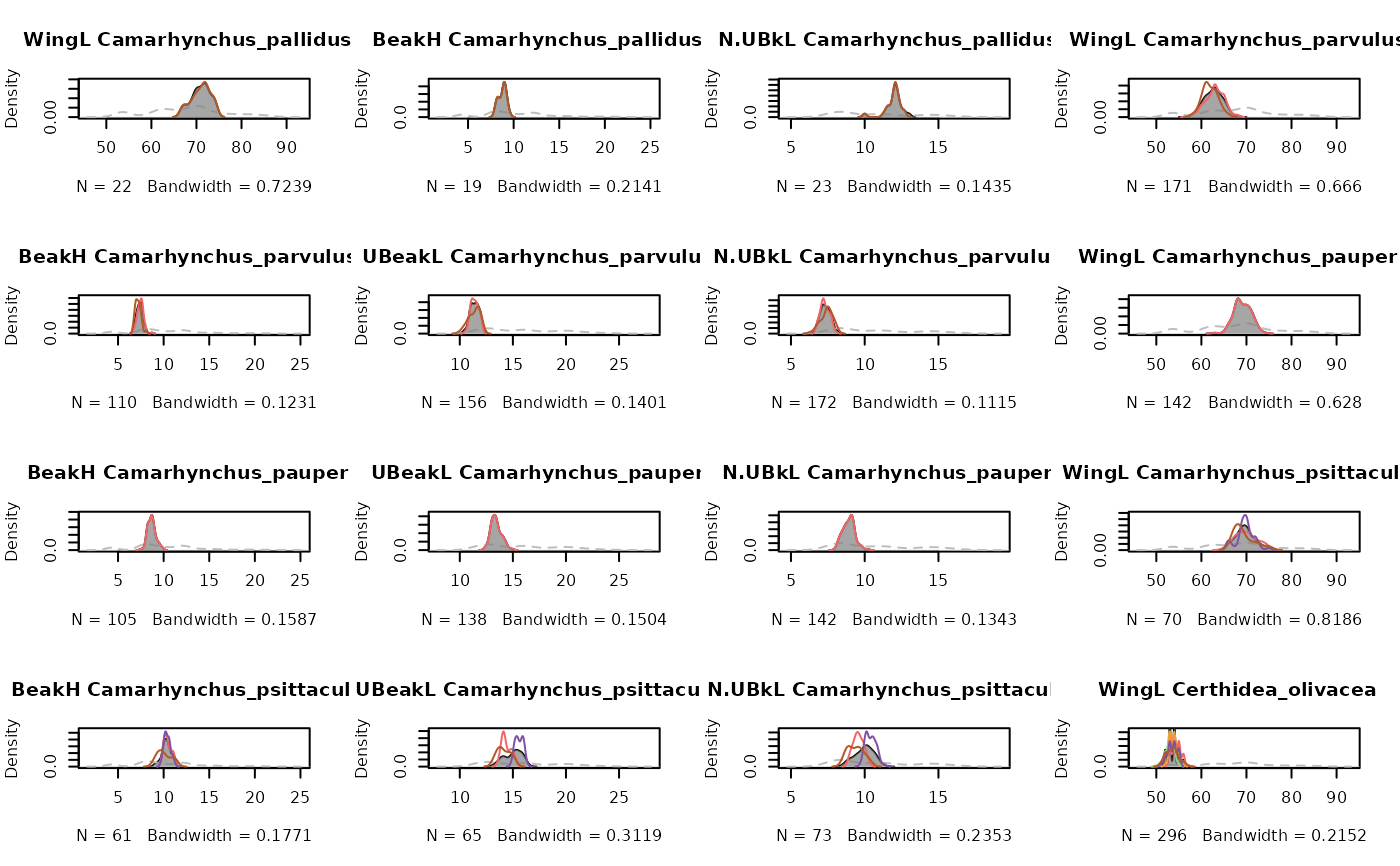
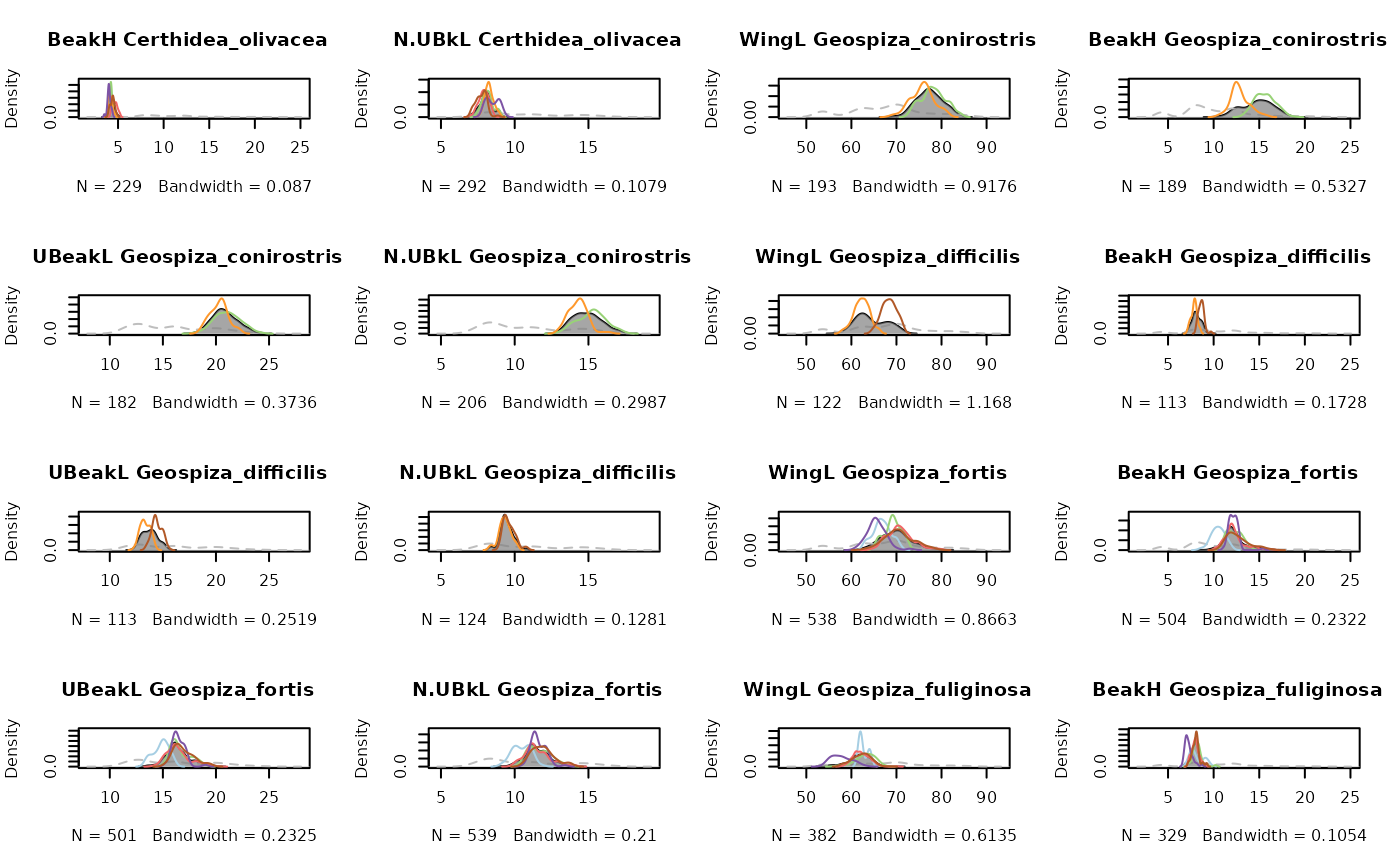
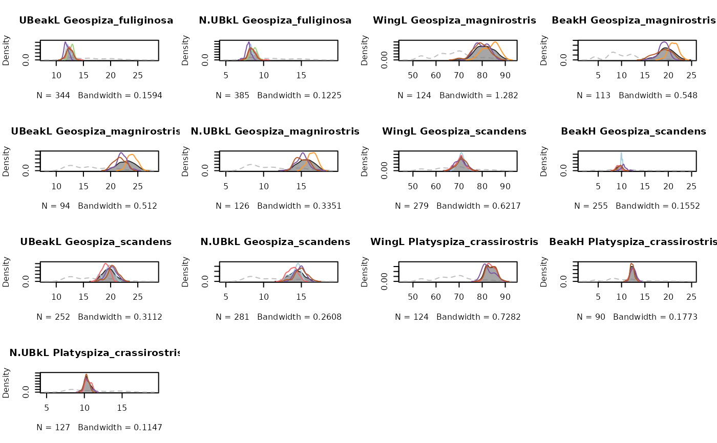
### First, let try the distribution for all populations
#of Darwin finches.
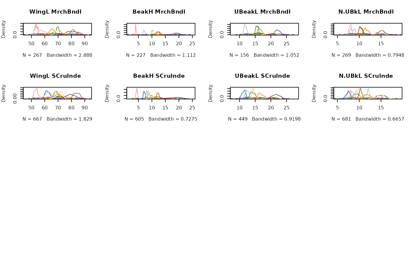
par(mfrow = c(4,4), cex = 0.5)
plotDistri(traits.finch, sp.finch, ind.plot.finch, ylim.cex = 3,
plot.ask = FALSE, multipanel = FALSE, leg = FALSE)
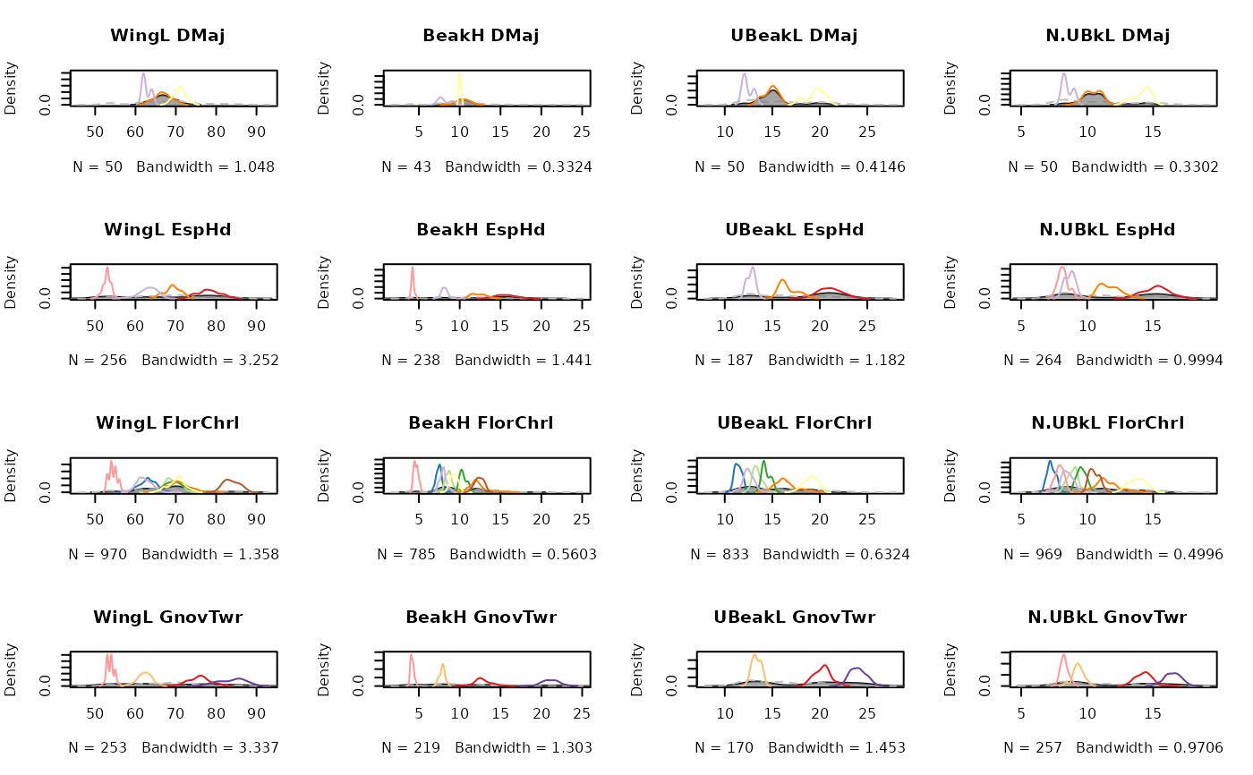
 ### Then we can inverse the second and the third arguments
#to plot the distribution for all finches species.
par(mfrow = c(4,4), cex = 0.5)
 plotDistri(traits.finch, ind.plot.finch, sp.finch, ylim.cex = 8,
plot.ask = FALSE, multipanel = FALSE, leg = FALSE)
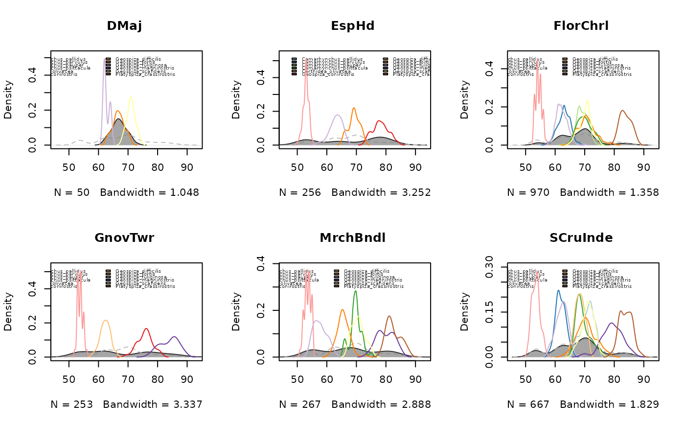
 ### Only one trait to plot using leg = TRUE to plot the legend
par(mfrow=c(2,3))
 plotDistri(as.matrix(traits.finch[,1]), ind.plot.finch, sp.finch,
ylim.cex=8, plot.ask = FALSE, multipanel = FALSE, leg = TRUE, cex.leg=0.5)
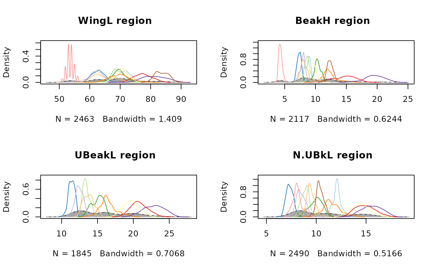
 ### You can also plot trait distribution for all species in the region
par(mfrow = c(1,1), cex = 1)
plotDistri(traits.finch, rep("region", times = dim(traits.finch)[1]),
sp.finch, ylim.cex = 6, plot.ask = FALSE, leg = FALSE)
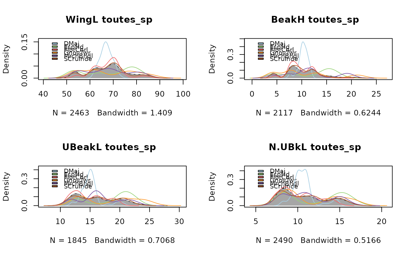
 ### You can also plot trait distribution for all sites
#without taking into account species identity
plotDistri(traits.finch, rep("toutes_sp", times = dim(traits.finch)[1]),
ind.plot.finch, ylim.cex = 3, plot.ask = FALSE)
 # }
# }