Skip to contents

Choosing reference databases for taxonomic assignment is not a matter of picking the single “best” one. Databases relate to each other in two fundamentally different ways, and confusing them leads to bad choices:

  • Nestedness (sequence derivation). Some databases incorporate sequences from others. Using two databases that share a common ancestor double-counts the same sequences and gives a false sense of corroboration.
  • Coverage overlap (parallel use). Some databases independently cover the same clade or marker. These are genuine alternatives — or complements when their markers differ.

This article maps both relationships from primary sources (official sites and the describing papers). Every derivation edge below traces to a sentence stating that one database is built from, incorporates, or re-annotates another. Where two databases merely cover the same organisms with independently curated sequences, that is coverage overlap, not derivation, and it is kept in a separate layer.

The sourced derivation table

Each row is a confirmed sequence-incorporation relationship, with the primary source. Nodes tagged (external) are upstream resources that are not themselves downloadable through dbpq.

Code
derivation <- tribble(
  ~from,          ~to,            ~what,                                  ~source,
  # ---- KSGP / GTDB+ lineage (KSGP 3.1, Bahram et al. 2025) ----
  "GTDB",         "GTDB_cleaned", "16S, domain-checked & deduplicated",   "KSGP 3.1 (2025)",
  "GTDB_cleaned", "GTDB+",        "prokaryote 16S backbone",              "KSGP 3.1 (2025)",
  "PR2",          "GTDB+",        "eukaryote 18S + plastid",              "KSGP 3.1 (2025)",
  "MIDORI2",      "GTDB+",        "mitochondrial SSU",                    "KSGP 3.1 (2025)",
  "GTDB+",        "KSGP",         "prokaryote backbone",                  "KSGP 3.1 (2025)",
  "SILVA",        "KSGP",         "Archaea 138.1, re-annotated",          "KSGP 3.1 (2025)",
  "Karst 2018",   "KSGP",         "near-full-length environmental SSU",   "KSGP 3.1 (2025)",
  # ---- Greengenes2 (McDonald et al. 2023) ----
  "GTDB",         "Greengenes2",  "r207 full-length 16S + taxonomy",      "Greengenes2 (2023)",
  "LTP",          "Greengenes2",  "Living Tree Project Jan 2022",         "Greengenes2 (2023)",
  "Karst 2018",   "Greengenes2",  "near-complete 16S",                    "Greengenes2 (2023)",
  "EMP500",       "Greengenes2",  "16S (Earth Microbiome Project)",       "Greengenes2 (2023)",
  # ---- LTPlus (Rossello-Mora et al. 2026) ----
  "LTP",          "LTPlus",       "type-strain backbone",                 "LTPlus (2026)",
  "SILVA",        "LTPlus",       "non-redundant 16S",                    "LTPlus (2026)",
  "GTDB",         "LTPlus",       "16S",                                  "LTPlus (2026)",
  "INSDc",        "LTPlus",       "best-quality NCBI 16S (2019-2025)",    "LTPlus (2026)",
  # ---- EUKARYOME (Tedersoo et al. 2024) ----
  "SILVA",        "Eukaryome",    "v138.1 SSU/LSU",                       "EUKARYOME (2024)",
  "PR2",          "Eukaryome",    "v4.14.1 SSU",                          "EUKARYOME (2024)",
  "UNITE",        "Eukaryome",    "v9.0 ITS",                             "EUKARYOME (2024)",
  "INSDc",        "Eukaryome",    "full-length (meta)genomic reads",      "EUKARYOME (2024)",
  # ---- INSDc (GenBank/EMBL/DDBJ) as the common root ----
  "INSDc",        "PR2",          "18S records (GenBank/EMBL/WGS)",       "PR2 documentation",
  "INSDc",        "SILVA",        "rRNA records",                         "SILVA",
  "INSDc",        "UNITE",        "ITS records",                          "UNITE",
  "INSDc",        "MIDORI2",      "mitochondrial records",                "MIDORI2 (2022)",
  "INSDc",        "MaarjAM",      "Glomeromycota SSU records",            "MaarjAM (2010)",
  "INSDc",        "RDP",          "16S records",                          "RDP",
  "INSDc",        "Diat.barcode", "rbcL records",                         "Diat.barcode",
  "INSDc",        "BOLD",         "barcode records (mirrored to INSDc)",  "BOLD"
)

# Annotation-only links: taxonomy/metadata transfer, NOT sequence incorporation.
annotation <- tribble(
  ~from,     ~to,   ~what,
  "SILVA",   "PR2", "taxonomy/metadata cross-reference",
  "EukRef",  "PR2", "expert taxonomic annotation",
  "EukRibo", "PR2", "taxonomic annotation"
)

knitr::kable(derivation, caption = "Confirmed sequence-derivation edges (source -> target).")
Confirmed sequence-derivation edges (source -> target).
from to what source
GTDB GTDB_cleaned 16S, domain-checked & deduplicated KSGP 3.1 (2025)
GTDB_cleaned GTDB+ prokaryote 16S backbone KSGP 3.1 (2025)
PR2 GTDB+ eukaryote 18S + plastid KSGP 3.1 (2025)
MIDORI2 GTDB+ mitochondrial SSU KSGP 3.1 (2025)
GTDB+ KSGP prokaryote backbone KSGP 3.1 (2025)
SILVA KSGP Archaea 138.1, re-annotated KSGP 3.1 (2025)
Karst 2018 KSGP near-full-length environmental SSU KSGP 3.1 (2025)
GTDB Greengenes2 r207 full-length 16S + taxonomy Greengenes2 (2023)
LTP Greengenes2 Living Tree Project Jan 2022 Greengenes2 (2023)
Karst 2018 Greengenes2 near-complete 16S Greengenes2 (2023)
EMP500 Greengenes2 16S (Earth Microbiome Project) Greengenes2 (2023)
LTP LTPlus type-strain backbone LTPlus (2026)
SILVA LTPlus non-redundant 16S LTPlus (2026)
GTDB LTPlus 16S LTPlus (2026)
INSDc LTPlus best-quality NCBI 16S (2019-2025) LTPlus (2026)
SILVA Eukaryome v138.1 SSU/LSU EUKARYOME (2024)
PR2 Eukaryome v4.14.1 SSU EUKARYOME (2024)
UNITE Eukaryome v9.0 ITS EUKARYOME (2024)
INSDc Eukaryome full-length (meta)genomic reads EUKARYOME (2024)
INSDc PR2 18S records (GenBank/EMBL/WGS) PR2 documentation
INSDc SILVA rRNA records SILVA
INSDc UNITE ITS records UNITE
INSDc MIDORI2 mitochondrial records MIDORI2 (2022)
INSDc MaarjAM Glomeromycota SSU records MaarjAM (2010)
INSDc RDP 16S records RDP
INSDc Diat.barcode rbcL records Diat.barcode
INSDc BOLD barcode records (mirrored to INSDc) BOLD

The derivation network

Hover a node to highlight its connections; arrows point from a source to the database that incorporates it. Square nodes are databases you can download with dbpq; round nodes are upstream (external) sources.

Code
library(visNetwork)

dbpq_dbs <- c(
  "UNITE", "SILVA", "PR2", "BOLD", "MaarjAM", "Eukaryome",
  "Greengenes2", "RDP", "MIDORI2", "Diat.barcode", "KSGP",
  "GTDB+", "GTDB_cleaned", "LTPlus"
)

all_nodes <- union(c(derivation$from, derivation$to), dbpq_dbs)

nodes <- tibble(id = all_nodes) |>
  mutate(
    group = if_else(id %in% dbpq_dbs, "dbpq database", "external source"),
    label = id
  )

edges <- derivation |>
  transmute(
    from, to,
    title = what,
    arrows = "to",
    color = "#6e2c9b"
  )

visNetwork(nodes, edges, height = "560px", width = "100%") |>
  visGroups(
    groupname = "dbpq database",
    shape = "box", color = "#10677c", font = list(color = "white")
  ) |>
  visGroups(
    groupname = "external source",
    shape = "dot", color = "#9aa0a6"
  ) |>
  visEdges(smooth = list(enabled = TRUE, type = "cubicBezier")) |>
  visNodes(font = list(size = 18)) |>
  visOptions(highlightNearest = list(enabled = TRUE, degree = 1, hover = TRUE)) |>
  visHierarchicalLayout(direction = "LR", sortMethod = "directed") |>
  visLegend(width = 0.15, position = "right", main = "Node type")

The derivation matrix

The same information as an adjacency matrix: a filled cell at row i, column j means “sequences from i are incorporated into j. Reading down a column tells you everything a database is built from; reading across a row tells you everywhere a database’s sequences end up. Annotation-only links (taxonomy transferred without sequences) are shown in a lighter shade to keep them distinct from true nestedness.

Code
lvls <- c(
  "INSDc", "GTDB", "Karst 2018", "LTP", "EMP500",
  "SILVA", "PR2", "UNITE", "MIDORI2", "EukRef", "EukRibo",
  "GTDB_cleaned", "GTDB+",
  "Eukaryome", "Greengenes2", "KSGP", "LTPlus",
  "MaarjAM", "RDP", "Diat.barcode", "BOLD"
)

mat <- bind_rows(
  derivation |> transmute(from, to, kind = "sequence incorporation"),
  annotation |> transmute(from, to, kind = "annotation only")
) |>
  mutate(
    from = factor(from, levels = lvls),
    to = factor(to, levels = rev(lvls))
  )

ggplot(mat, aes(x = from, y = to, fill = kind)) +
  geom_tile(color = "white", linewidth = 0.6) +
  scale_fill_manual(
    values = c(
      "sequence incorporation" = "#3e135a",
      "annotation only" = "#c9b3da"
    ),
    name = NULL
  ) +
  labs(
    x = "Source (sequences come FROM)",
    y = "Target (... are incorporated INTO)",
    title = "Derivation adjacency matrix"
  ) +
  coord_fixed() +
  theme_minimal(base_size = 11) +
  theme(
    axis.text.x = element_text(angle = 45, hjust = 1),
    panel.grid = element_line(color = "grey92"),
    legend.position = "top"
  )

Three structural facts pop out of the matrix:

  • INSDc (GenBank/EMBL/DDBJ) is the common root. Almost every database ultimately draws its raw sequences from INSDc — “independent” means independently curated, never sequence-disjoint at the source.
  • KSGP sits at the deepest point. It pulls from GTDB+, which itself pulls from GTDB, PR2 and MIDORI2 — a three-level chain.
  • Eukaryome, Greengenes2 and LTPlus are convergence nodes. Several otherwise independent databases flow into each of them — Eukaryome merges SILVA, PR2 and UNITE, while Greengenes2 and LTPlus both synthesise the prokaryote 16S space from GTDB and SILVA/LTP.

Coverage overlap: which databases are alternatives

Nestedness tells you which databases not to treat as independent evidence. Coverage tells you which databases are interchangeable or complementary for a given target. The heatmap below maps each database to the clades it can assign, annotated with its marker. Two databases in the same row (same clade) are alternatives; if their markers differ they are complementary.

Code
coverage <- tribble(
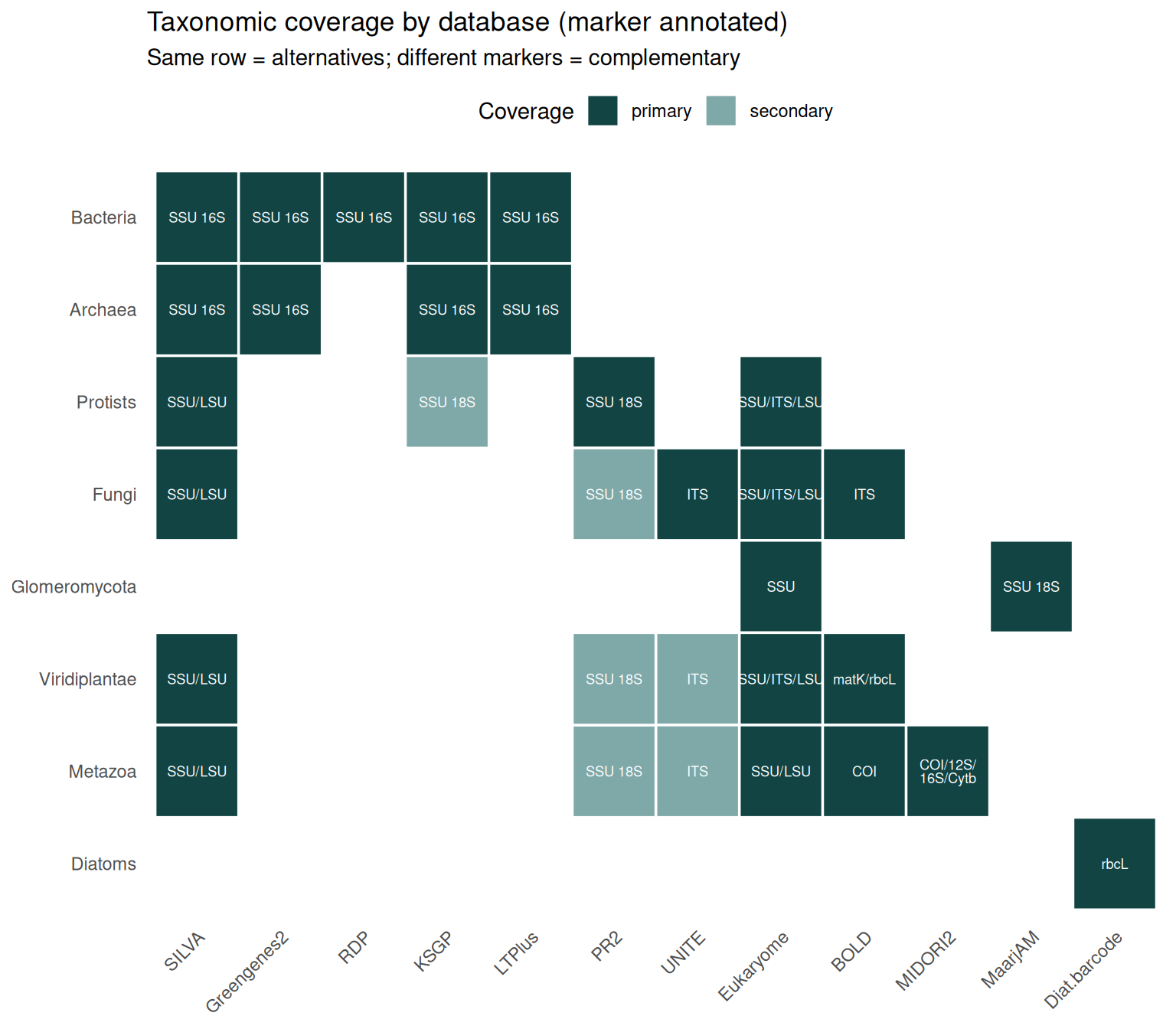
  ~database,       ~clade,            ~marker,    ~role,
  "SILVA",         "Bacteria",        "SSU 16S",  "primary",
  "Greengenes2",   "Bacteria",        "SSU 16S",  "primary",
  "RDP",           "Bacteria",        "SSU 16S",  "primary",
  "KSGP",          "Bacteria",        "SSU 16S",  "primary",
  "LTPlus",        "Bacteria",        "SSU 16S",  "primary",
  "SILVA",         "Archaea",         "SSU 16S",  "primary",
  "Greengenes2",   "Archaea",         "SSU 16S",  "primary",
  "KSGP",          "Archaea",         "SSU 16S",  "primary",
  "LTPlus",        "Archaea",         "SSU 16S",  "primary",
  "PR2",           "Protists",        "SSU 18S",  "primary",
  "SILVA",         "Protists",        "SSU/LSU",  "primary",
  "Eukaryome",     "Protists",        "SSU/ITS/LSU", "primary",
  "UNITE",         "Fungi",           "ITS",      "primary",
  "SILVA",         "Fungi",           "SSU/LSU",  "primary",
  "Eukaryome",     "Fungi",           "SSU/ITS/LSU", "primary",
  "BOLD",          "Fungi",           "ITS",      "primary",
  "MaarjAM",       "Glomeromycota",   "SSU 18S",  "primary",
  "Eukaryome",     "Glomeromycota",   "SSU",      "primary",
  "SILVA",         "Viridiplantae",   "SSU/LSU",  "primary",
  "Eukaryome",     "Viridiplantae",   "SSU/ITS/LSU", "primary",
  "BOLD",          "Viridiplantae",   "matK/rbcL", "primary",
  "SILVA",         "Metazoa",         "SSU/LSU",  "primary",
  "Eukaryome",     "Metazoa",         "SSU/LSU",  "primary",
  "BOLD",          "Metazoa",         "COI",      "primary",
  "MIDORI2",       "Metazoa",         "COI/12S/\n16S/Cytb", "primary",
  "Diat.barcode",  "Diatoms",         "rbcL",     "primary",
  # secondary (contamination-filtering) coverage
  "UNITE",         "Viridiplantae",   "ITS",      "secondary",
  "UNITE",         "Metazoa",         "ITS",      "secondary",
  "PR2",           "Metazoa",         "SSU 18S",  "secondary",
  "PR2",           "Fungi",           "SSU 18S",  "secondary",
  "PR2",           "Viridiplantae",   "SSU 18S",  "secondary",
  "KSGP",          "Protists",        "SSU 18S",  "secondary"
)

clade_lvls <- c(
  "Bacteria", "Archaea", "Protists", "Fungi", "Glomeromycota",
  "Viridiplantae", "Metazoa", "Diatoms"
)
db_lvls <- c(
  "SILVA", "Greengenes2", "RDP", "KSGP", "LTPlus", "PR2", "UNITE",
  "Eukaryome", "BOLD", "MIDORI2", "MaarjAM", "Diat.barcode"
)

coverage <- coverage |>
  mutate(
    clade = factor(clade, levels = rev(clade_lvls)),
    database = factor(database, levels = db_lvls)
  )

ggplot(coverage, aes(x = database, y = clade)) +
  geom_tile(aes(fill = role), color = "white", linewidth = 0.6) +
  geom_text(aes(label = marker), size = 2.4, color = "white", lineheight = 0.8) +
  scale_fill_manual(
    values = c("primary" = "#124444", "secondary" = "#7fa8a8"),
    name = "Coverage"
  ) +
  labs(
    x = NULL, y = NULL,
    title = "Taxonomic coverage by database (marker annotated)",
    subtitle = "Same row = alternatives; different markers = complementary"
  ) +
  theme_minimal(base_size = 11) +
  theme(
    axis.text.x = element_text(angle = 45, hjust = 1),
    panel.grid = element_blank(),
    legend.position = "top"
  )

Putting it together: practical guidance

Combine the two layers when designing an assignment strategy:

  • Don’t stack nested databases as independent evidence. Eukaryome already contains SILVA, PR2 and UNITE; running UNITE and Eukaryome on the same fungal ITS reads is not two independent opinions. Likewise KSGP, Greengenes2 and LTPlus all draw on GTDB and SILVA/LTP, so treat them as variations on one prokaryote 16S resource, not independent corroboration.
  • Do combine genuinely independent, complementary databases. For a soil eukaryote survey: UNITE (fungal ITS) + MaarjAM (AMF SSU, a clade UNITE under-resolves) + PR2 (protist SSU) cover different clades and markers with independent curation.
  • Pick the marker-matched primary database per clade from the coverage heatmap, then use secondary coverage (lighter cells) only to flag and remove off-target reads, not to assign them at fine rank.

Sources

Derivation relationships were verified against the following primary sources (June 2026):