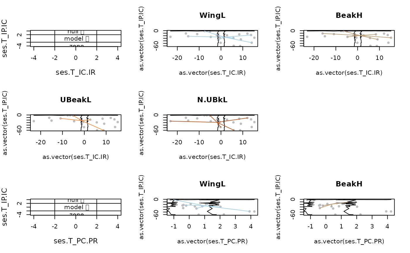
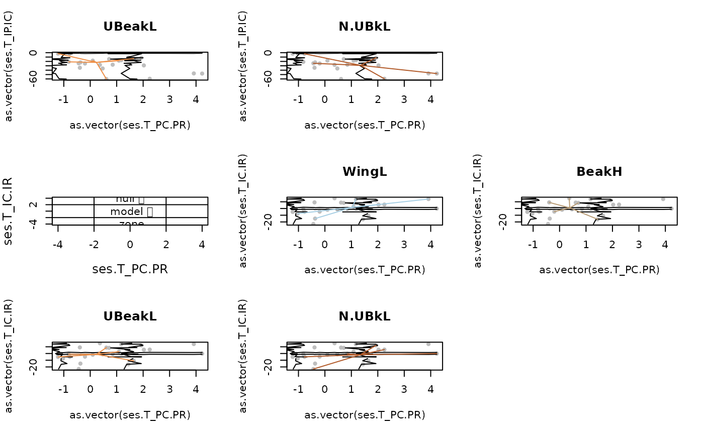
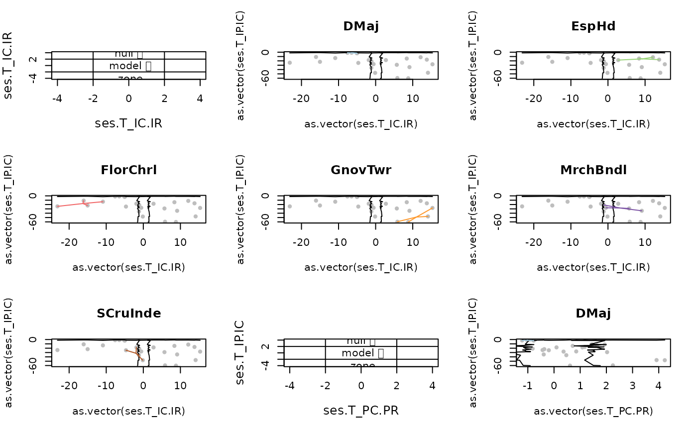
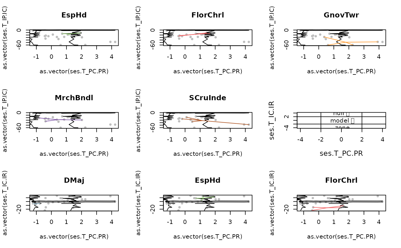
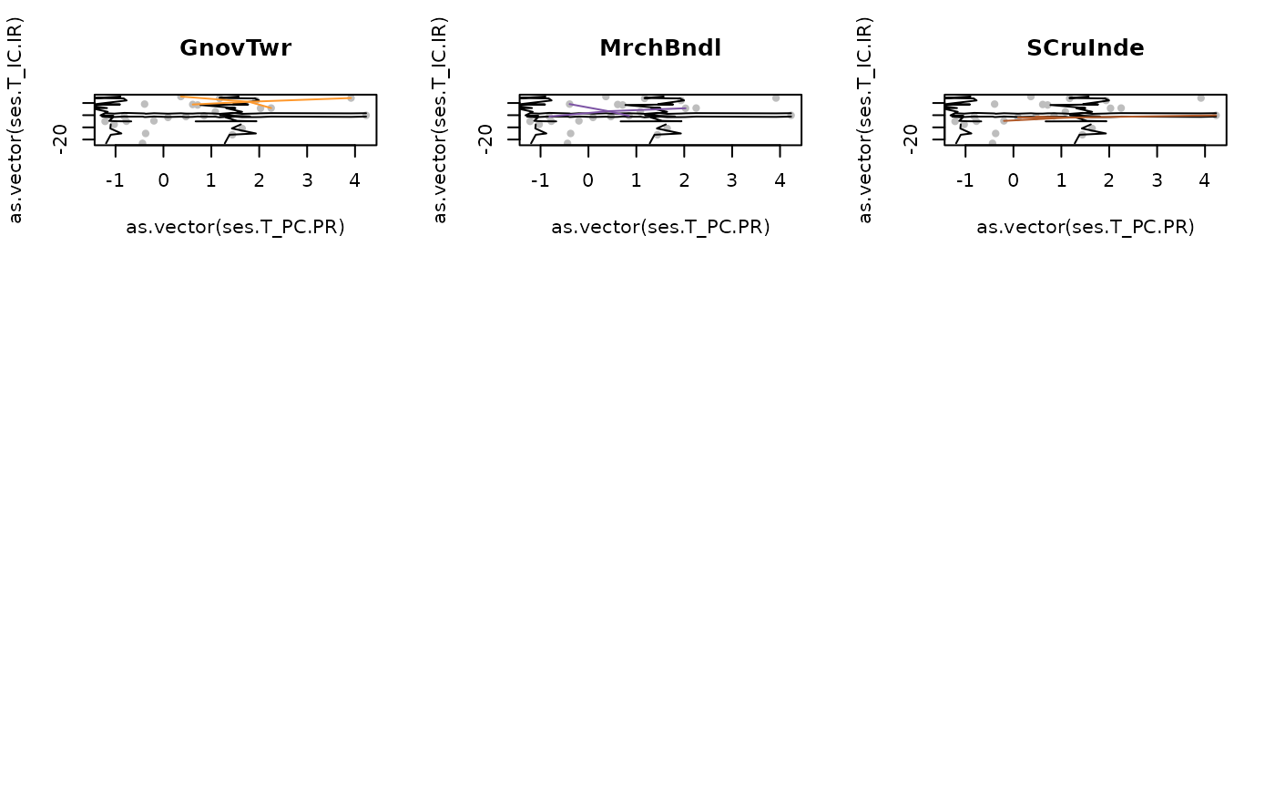
Plot the bivariate relationships between T-statistics

Plot the bivariate relationships between the three T-statistics namely T_IP.IC, T_IC.IR and T_PC.PR.

Usage

plotCorTstats(tstats = NULL, val.quant = c(0.025, 0.975), 
  add.text =  FALSE, bysite =  FALSE, col.obj = NULL, plot.ask = TRUE, 
  multipanel = TRUE, ...)

Arguments

tstats

The list resulting from the function Tstats.

val.quant

Numeric vector of length 2, giving the quantile to calculate confidence interval. By default val.quant = c(0.025,0.975) for a bilateral test with alpha = 5%.

add.text

Logical value; Add text or not.

bysite

Logical value; plot per site or by traits.

col.obj

Vector of colors for object (either traits or sites).

plot.ask

Logical value; Ask for new plot or not.

multipanel

Logical value. If TRUE divides the device to shown several traits graphics in the same device.

...

Any additional arguments are passed to the plot function creating the core of the plot and can be used to adjust the look of resulting graph.

Value

None; used for the side-effect of producing a plot.

Author

Adrien Taudiere

See also

Tstats; plot.Tstats; plotSESvar

Examples

  data(finch.ind)
  res.finch <- Tstats(traits.finch, ind.plot = ind.plot.finch, 
  sp = sp.finch, nperm = 9)
#> Warning: This function exclude 1137 Na values
#> [1] "creating null models"
#> [1] "8.33 %"
#> [1] "16.67 %"
#> [1] "25 %"
#> [1] "33.33 %"
#> [1] "41.63 %"
#> [1] "49.97 %"
#> [1] "58.3 %"
#> [1] "66.63 %"
#> [1] "74.93 %"
#> [1] "83.27 %"
#> [1] "91.6 %"
#> [1] "99.93 %"
#> [1] "calculation of Tstats using null models"
#> [1] "8.33 %"
#> [1] "16.67 %"
#> [1] "25 %"
#> [1] "33.33 %"
#> [1] "41.63 %"
#> [1] "49.97 %"
#> [1] "58.3 %"
#> [1] "66.63 %"
#> [1] "74.93 %"
#> [1] "83.27 %"
#> [1] "91.6 %"
#> [1] "99.93 %"
  
  if (FALSE) { # \dontrun{
    plotCorTstats(res.finch, bysite = FALSE)
    plotCorTstats(res.finch, bysite = TRUE)
  } # }