Computing observed T-statistics (T for Traits) and null expectations.
Tstats.RdComputing observed T-statistics (T for Traits) as three ratios of variance, namely T_IP.IC, T_IC.IR and T_PC.PR. This function can also return the distribution of this three statistics under null models.
Usage
Tstats(traits, ind.plot, sp, SE = 0, reg.pool = NULL,
  SE.reg.pool = NULL, nperm = 99, printprogress = TRUE,
  independantTraits = TRUE)

  sum_Tstats(x, val.quant = c(0.025, 0.975), type = "all")

  ses.Tstats(x, val.quant = c(0.025, 0.975))

  # S3 method for class 'Tstats'
barplot(height, val.quant = c(0.025, 0.975),
  col.index = c("red", "purple", "olivedrab3", "white"), ylim = NULL, ...)

  # S3 method for class 'Tstats'
plot(x, type = "normal", col.index = c("red", "purple", "olivedrab3"),
  add.conf = TRUE, color.cond = TRUE, val.quant = c(0.025, 0.975), ...)

  # S3 method for class 'Tstats'
print(x, ...)

  # S3 method for class 'Tstats'
summary(object, ...)
Arguments
- traits
Individual Matrix of traits with traits in columns. For one trait, use as.matrix().
- ind.plot
Factor defining the name of the plot in which the individual is.
- sp
Factor defining the species which the individual belong to.
- SE
A single value or vector of standard errors associated with each traits. Especially allow to handle measurement errors. Not used with populational null model.
- reg.pool
Regional pool data for traits. If not informed, 'traits' is considered as the regional pool. This matrix need to be larger (more rows) than the matrix "traits". Use only for null model 2 (regional.ind).
- SE.reg.pool
A single value or vector of standard errors associated with each traits in each regional pool. Use only if reg.pool is used. Need to have the same dimension as reg.pool.
- nperm
Number of permutations. If NULL, only observed values are returned;
- printprogress
Logical value; print progress during the calculation or not.
- independantTraits
Logical value (default: TRUE). If independantTraits is true (default), each traits is sample independently in null models, if not, each lines of the matrix are randomized, keeping the relation (and trade-off) among traits.
- x
An object of class Tstats.
- height
An object of class Tstats.
- object
An object of class Tstats.
- val.quant
Numeric vectors of length 2, giving the quantile to calculation confidence interval. By default val.quant = c(0.025,0.975) for a bilateral test with alpha = 5%.
- ylim
Numeric vectors of length 2, giving the y coordinates range
- col.index
A vector of three color correspond to the three T-statistics.
- color.cond
Logical value; If color.cond = TRUE, color points indicate T-statistics values significatively different from the null model and grey points are not different from null model.
- type
For the plot function, type of plot. Possible type = "simple", "simple_range", "normal", "barplot" and "bytraits". For the summary function, type of summary statistics. Either "binary", "percent", "p.value", "site" or "all".
- add.conf
Logical value; Add confidence intervals or not.
- ...
Any additional arguments are passed to the plot function creating the core of the plot and can be used to adjust the look of resulting graph. See
plot.listofindexfor more arguments.
Details
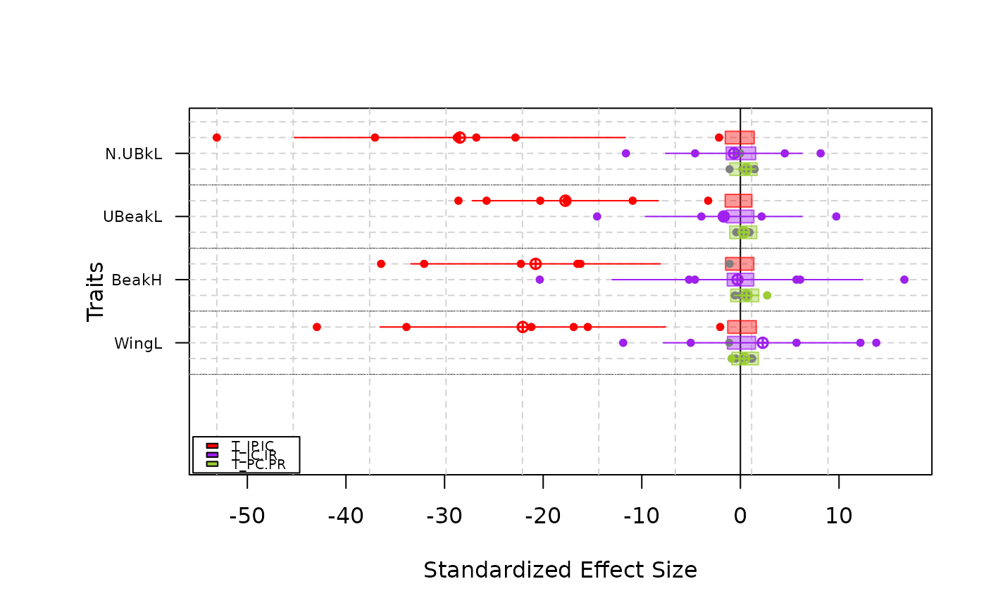
S3 method plot:
-Normal type plot means, standard deviations, ranges and confidence intervals of T-statistics.
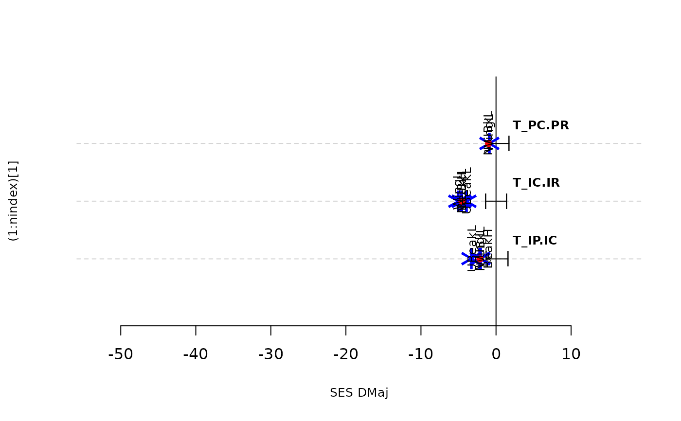
-Simple_range type plot means, standard deviations and range of T-statistics
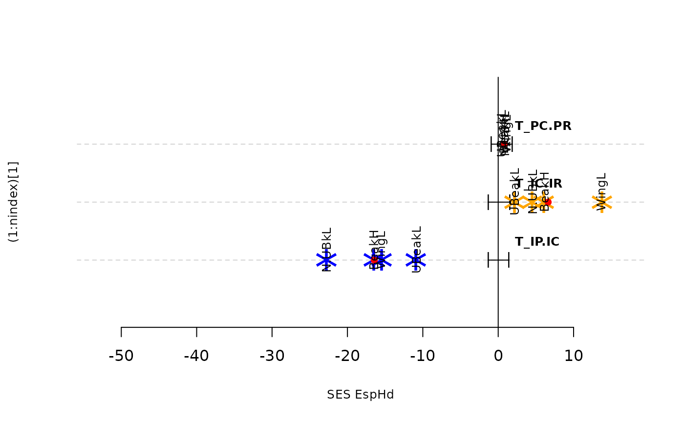
-Simple type plot T-statistics for each site and traits and the mean confidence intervals by traits
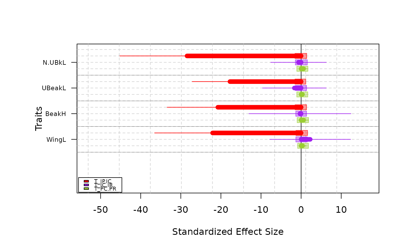
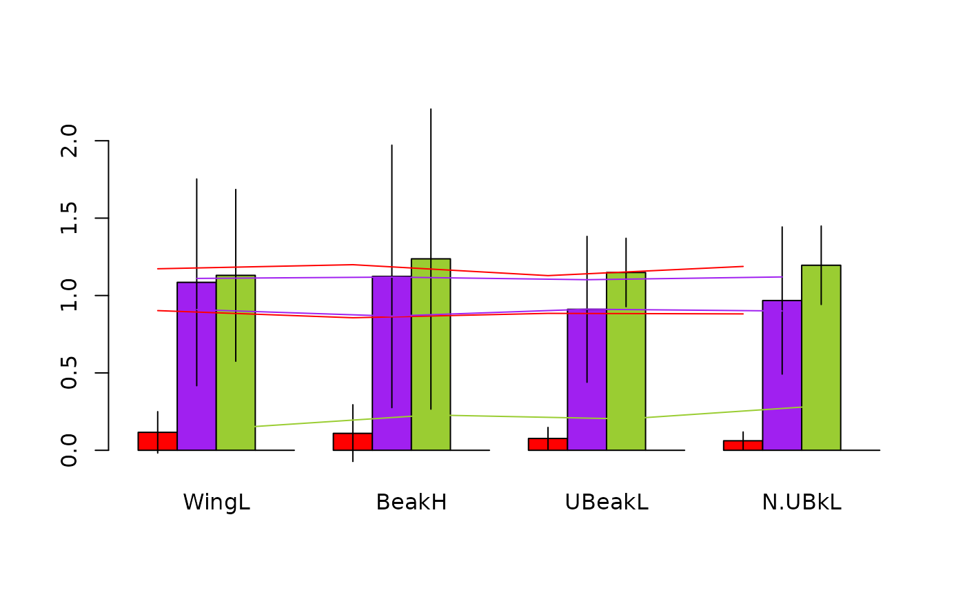
-Barplot type plot means, standard deviations and confidence intervals of T-statistics in a barplot fashion
-Bysites type plot each metrics for each sites
-Bytraits type plot each metrics for each traits
S3 method print: print the structure if the object of class Tstats
S3 method summary: print the summary statistics of the three T-statistics
Method summary sum_Tstats:
-Binary type only test if a T-statistics is significatively different from the null expectation for each trait.
-Percent type determine the percentage of sites were the T-statistics is significatively different from the null expectation for each trait. Asterix shows global significance of the test.
-P-value type determine the p-value (two unilateral tests) of the T-statistics for each trait and sites.
-Site type allows to know in which sites T-statistics deviate from the null expectation.
-All type do all the precedent type of summary.
Value
A list of statistics:
- Tstats$T_IP.IC
Observed ratio between variance of individuals in populations and individuals in communities
- Tstats$T_IC.IR
Observed ratio between variance of individuals in communities and individuals in the region
- Tstats$T_PC.PR
Observed ratio between variance of populations in communities and populations in the region
- $Tstats$T_IP.IC_nm
If nperm is numeric; Result of simulation for T_IP.IC
- $Tstats$T_IC.IR_nm
If nperm is numeric; Result of simulation for T_IC.IR
- $Tstats$T_PC.PR_nm
If nperm is numeric; Result of simulation for T_PC.PR
- $variances$var_IP
variance of individuals within populations
- $variances$var_PC
variance of populations within communities
- $variances$var_CR
variance of communities within the region
- $variances$var_IC
variance of individuals within communities
- $variances$var_PR
variance of populations within the region
- $variances$var_IR
variance of individuals within the region
- $variances$var_IP_nm1
variance of individuals within populations in null model 1
- $variances$var_PC_nm2sp
variance of populations within communities in null model 2sp
- $variances$var_IC_nm1
variance of communities within the region in null model 1
- $variances$var_IC_nm2
variance of individuals within communities in null model 2
- $variances$var_PR_nm2sp
variance of populations within the region in null model 2sp
- $variances$var_IR_nm2
variance of individuals within the region in null model 2
- $traits
traits data
- $ind.plot
name of the plot in which the individual is
- $sp
groups (e.g. species) which the individual belong to
- $call
call of the function Tstats
References
Violle, Cyrille, Brian J. Enquist, Brian J. McGill, Lin Jiang, Cecile H. Albert, Catherine Hulshof, Vincent Jung, et Julie Messier. 2012. The return of the variance: intraspecific variability in community ecology. Trends in Ecology & Evolution 27 (4): 244-252. doi:10.1016/j.tree.2011.11.014.
Examples
data(finch.ind)
# \donttest{
res.finch <- Tstats(traits.finch, ind.plot = ind.plot.finch,
sp = sp.finch, nperm = 9, printprogress = FALSE)
#> Warning: This function exclude 1137 Na values
res.finch
#> ##################
#> # T-statistics #
#> ##################
#> class: Tstats
#> $call: Tstats(traits = traits.finch, ind.plot = ind.plot.finch, sp = sp.finch,
#> nperm = 9, printprogress = FALSE)
#>
#> ###############
#> $Tstats: list of observed and null T-statistics
#>
#> Observed values
#> $T_IP.IC: ratio of within-population variance to total within-community variance
#> $T_IC.IR: community-wide variance relative to the total variance in the regional pool
#> $T_PC.PR: inter-community variance relative to the total variance in the regional pool
#>
#> Null values, number of permutations: 9
#> $T_IP.IC_nm: distribution of T_IP.IC value under the null model local
#> $T_IC.IR_nm: distribution of T_IC.IR value under the null model regional.ind
#> $T_PC.PR_nm: distribution of T_PC.PR value under the null model regional.pop
#>
#> ###############
#> $variances: list of observed and null variances
#>
#> ###############
#> data used
#> data class dim content
#> 1 $traits matrix 2513,4 traits data
#> 2 $ind.plot factor 2513 name of the plot in which the individual is
#> 3 $sp factor 2513 individuals' groups (e.g. species)
#>
#> ###############
#> others
#> $namestraits: 4 traits
#> [1] "WingL" "BeakH" "UBeakL" "N.UBkL"
#>
#> $nb.ind_plot:
#> ind.plot
#> DMaj EspHd FlorChrl GnovTwr MrchBndl SCruInde
#> 50 267 981 258 270 687
#>
#Tstats class is associated to S3 methods plot, barplot and summary
plot(res.finch)
 plot(res.finch, type = "simple")
 plot(res.finch, type = "simple_range")
 plot(res.finch, type = "barplot")
 plot(res.finch, type = "bysites")
 plot(res.finch, type = "bytraits")
 sum_Tstats(res.finch, type = "binary")
#> WingL BeakH UBeakL N.UBkL
#> T_IP.IC.inf TRUE TRUE TRUE TRUE
#> T_IP.IC.sup FALSE FALSE FALSE FALSE
#> T_IC.IR.inf FALSE FALSE TRUE FALSE
#> T_IC.IR.sup TRUE FALSE FALSE FALSE
#> T_PC.PR.inf FALSE NA NA FALSE
#> T_PC.PR.sup TRUE FALSE FALSE FALSE
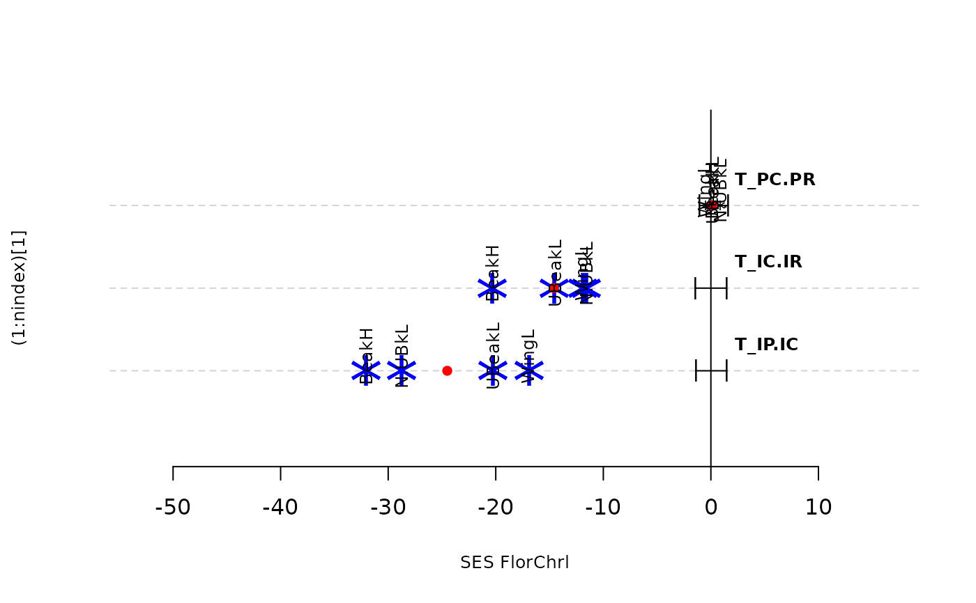
sum_Tstats(res.finch, type = "site")
#> WingL
#> T_IP.IC.inf "DMaj EspHd FlorChrl GnovTwr MrchBndl SCruInde"
#> T_IP.IC.sup "H0 not rejected"
#> T_IC.IR.inf "DMaj EspHd FlorChrl GnovTwr MrchBndl SCruInde"
#> T_IC.IR.sup "EspHd GnovTwr MrchBndl"
#> T_PC.PR.inf "DMaj"
#> T_PC.PR.sup "H0 not rejected"
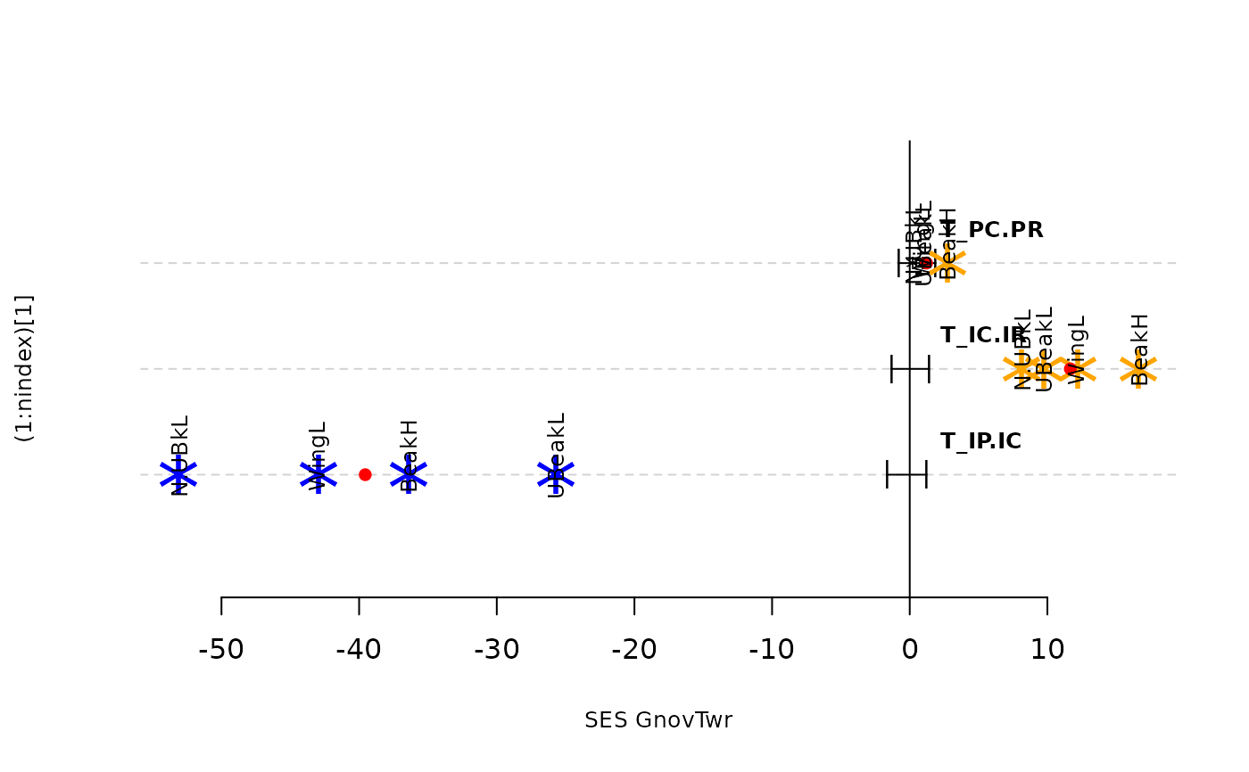
#> BeakH
#> T_IP.IC.inf "EspHd FlorChrl GnovTwr MrchBndl SCruInde"
#> T_IP.IC.sup "H0 not rejected"
#> T_IC.IR.inf "EspHd FlorChrl GnovTwr MrchBndl SCruInde"
#> T_IC.IR.sup "EspHd GnovTwr MrchBndl"
#> T_PC.PR.inf "H0 not rejected"
#> T_PC.PR.sup "GnovTwr"
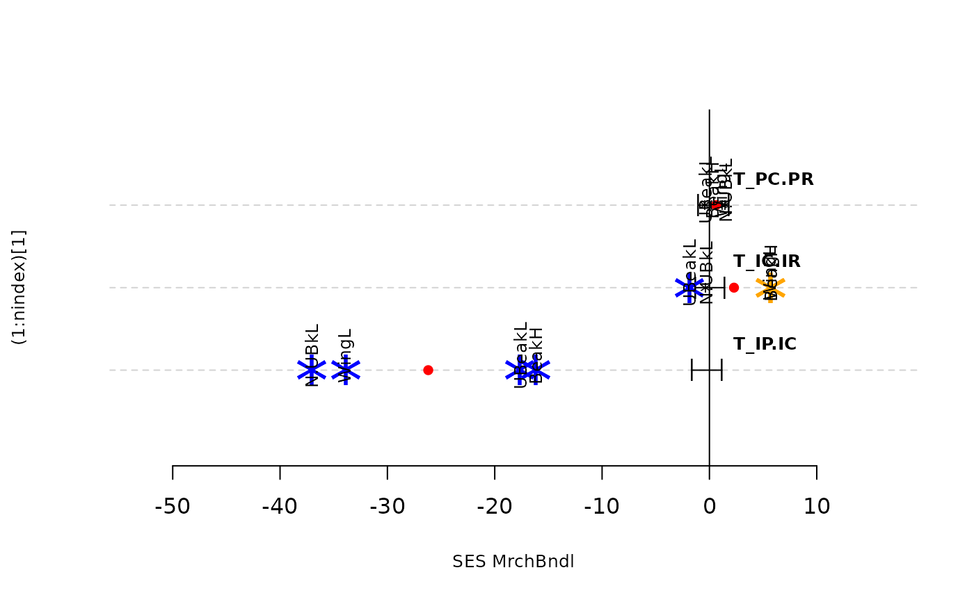
#> UBeakL
#> T_IP.IC.inf "DMaj EspHd FlorChrl GnovTwr MrchBndl SCruInde"
#> T_IP.IC.sup "H0 not rejected"
#> T_IC.IR.inf "DMaj EspHd FlorChrl GnovTwr MrchBndl SCruInde"
#> T_IC.IR.sup "EspHd GnovTwr"
#> T_PC.PR.inf "H0 not rejected"
#> T_PC.PR.sup "H0 not rejected"
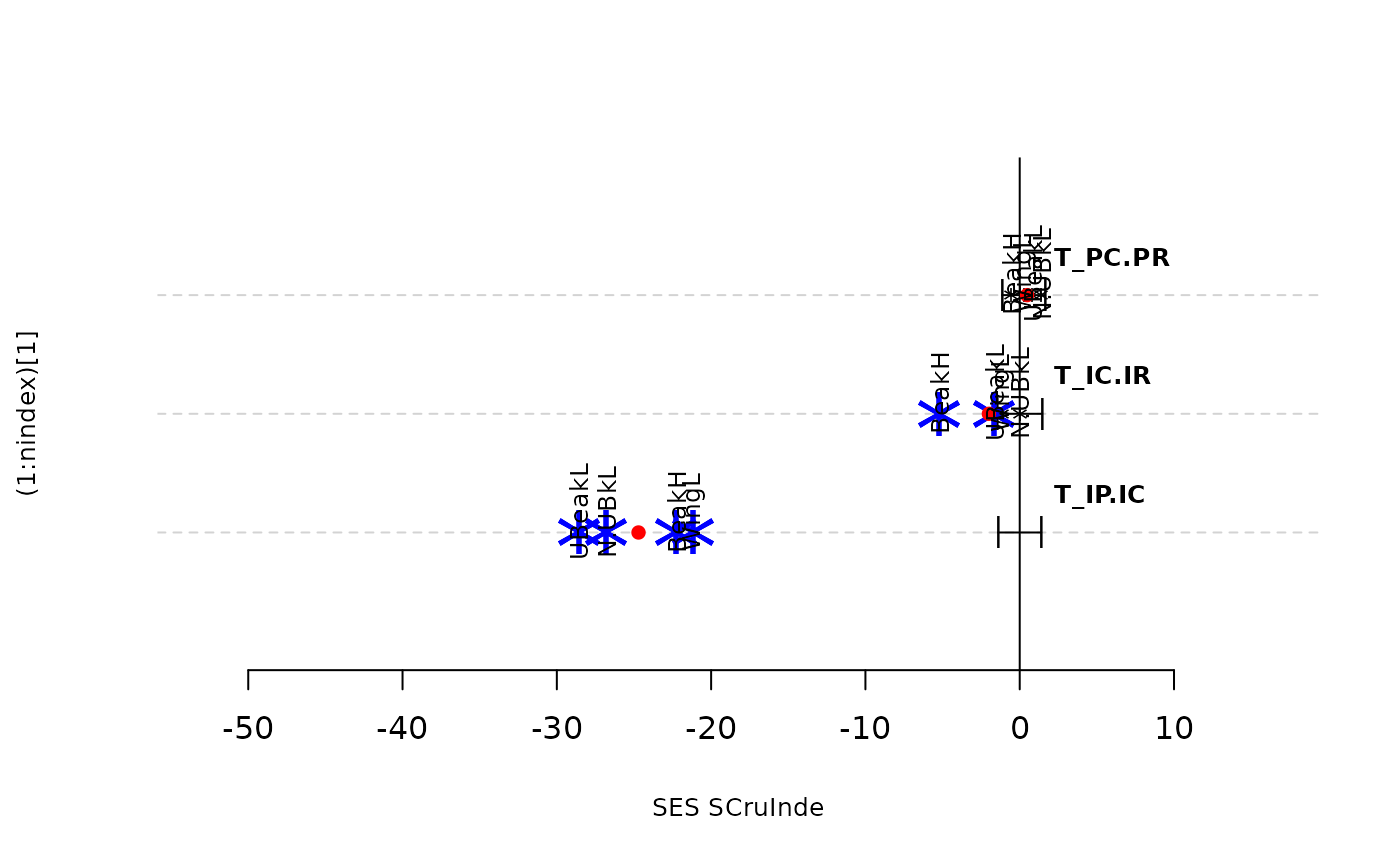
#> N.UBkL
#> T_IP.IC.inf "DMaj EspHd FlorChrl GnovTwr MrchBndl SCruInde"
#> T_IP.IC.sup "H0 not rejected"
#> T_IC.IR.inf "DMaj EspHd FlorChrl GnovTwr MrchBndl SCruInde"
#> T_IC.IR.sup "EspHd GnovTwr"
#> T_PC.PR.inf "H0 not rejected"
#> T_PC.PR.sup "H0 not rejected"
sum_Tstats(res.finch, type = "p.value")
#> WingL BeakH UBeakL N.UBkL
#> T_IP.IC.inf DMaj 0.1 0.2 0.1 0.1
#> T_IP.IC.inf EspHd 0.1 0.1 0.1 0.1
#> T_IP.IC.inf FlorChrl 0.1 0.1 0.1 0.1
#> T_IP.IC.inf GnovTwr 0.1 0.1 0.1 0.1
#> T_IP.IC.inf MrchBndl 0.1 0.1 0.1 0.1
#> T_IP.IC.inf SCruInde 0.1 0.1 0.1 0.1
#> T_IP.IC.sup DMaj 1.0 0.9 1.0 1.0
#> T_IP.IC.sup EspHd 1.0 1.0 1.0 1.0
#> T_IP.IC.sup FlorChrl 1.0 1.0 1.0 1.0
#> T_IP.IC.sup GnovTwr 1.0 1.0 1.0 1.0
#> T_IP.IC.sup MrchBndl 1.0 1.0 1.0 1.0
#> T_IP.IC.sup SCruInde 1.0 1.0 1.0 1.0
#> T_IC.IR.inf DMaj 0.1 0.1 0.1 0.1
#> T_IC.IR.inf EspHd 1.0 1.0 1.0 1.0
#> T_IC.IR.inf FlorChrl 0.1 0.1 0.1 0.1
#> T_IC.IR.inf GnovTwr 1.0 1.0 1.0 1.0
#> T_IC.IR.inf MrchBndl 1.0 1.0 0.1 0.5
#> T_IC.IR.inf SCruInde 0.2 0.1 0.1 0.4
#> T_IC.IR.sup DMaj 1.0 1.0 1.0 1.0
#> T_IC.IR.sup EspHd 0.1 0.1 0.1 0.1
#> T_IC.IR.sup FlorChrl 1.0 1.0 1.0 1.0
#> T_IC.IR.sup GnovTwr 0.1 0.1 0.1 0.1
#> T_IC.IR.sup MrchBndl 0.1 0.1 1.0 0.6
#> T_IC.IR.sup SCruInde 0.9 1.0 1.0 0.7
#> T_PC.PR.inf DMaj 0.1 0.1 0.2 0.2
#> T_PC.PR.inf EspHd 0.9 0.9 0.8 0.9
#> T_PC.PR.inf FlorChrl 0.5 0.7 0.7 0.8
#> T_PC.PR.inf GnovTwr 0.9 0.9 0.9 0.7
#> T_PC.PR.inf MrchBndl 0.9 0.7 0.5 0.9
#> T_PC.PR.inf SCruInde 0.7 0.5 0.8 0.9
#> T_PC.PR.sup DMaj 1.0 0.1 0.1 0.9
#> T_PC.PR.sup EspHd 0.2 0.2 0.3 0.2
#> T_PC.PR.sup FlorChrl 0.6 0.4 0.4 0.3
#> T_PC.PR.sup GnovTwr 0.2 0.1 0.2 0.4
#> T_PC.PR.sup MrchBndl 0.2 0.4 0.6 0.2
#> T_PC.PR.sup SCruInde 0.4 0.6 0.3 0.2
barplot(res.finch)
sum_Tstats(res.finch, type = "binary")
#> WingL BeakH UBeakL N.UBkL
#> T_IP.IC.inf TRUE TRUE TRUE TRUE
#> T_IP.IC.sup FALSE FALSE FALSE FALSE
#> T_IC.IR.inf FALSE FALSE TRUE FALSE
#> T_IC.IR.sup TRUE FALSE FALSE FALSE
#> T_PC.PR.inf FALSE NA NA FALSE
#> T_PC.PR.sup TRUE FALSE FALSE FALSE
sum_Tstats(res.finch, type = "site")
#> WingL
#> T_IP.IC.inf "DMaj EspHd FlorChrl GnovTwr MrchBndl SCruInde"
#> T_IP.IC.sup "H0 not rejected"
#> T_IC.IR.inf "DMaj EspHd FlorChrl GnovTwr MrchBndl SCruInde"
#> T_IC.IR.sup "EspHd GnovTwr MrchBndl"
#> T_PC.PR.inf "DMaj"
#> T_PC.PR.sup "H0 not rejected"
#> BeakH
#> T_IP.IC.inf "EspHd FlorChrl GnovTwr MrchBndl SCruInde"
#> T_IP.IC.sup "H0 not rejected"
#> T_IC.IR.inf "EspHd FlorChrl GnovTwr MrchBndl SCruInde"
#> T_IC.IR.sup "EspHd GnovTwr MrchBndl"
#> T_PC.PR.inf "H0 not rejected"
#> T_PC.PR.sup "GnovTwr"
#> UBeakL
#> T_IP.IC.inf "DMaj EspHd FlorChrl GnovTwr MrchBndl SCruInde"
#> T_IP.IC.sup "H0 not rejected"
#> T_IC.IR.inf "DMaj EspHd FlorChrl GnovTwr MrchBndl SCruInde"
#> T_IC.IR.sup "EspHd GnovTwr"
#> T_PC.PR.inf "H0 not rejected"
#> T_PC.PR.sup "H0 not rejected"
#> N.UBkL
#> T_IP.IC.inf "DMaj EspHd FlorChrl GnovTwr MrchBndl SCruInde"
#> T_IP.IC.sup "H0 not rejected"
#> T_IC.IR.inf "DMaj EspHd FlorChrl GnovTwr MrchBndl SCruInde"
#> T_IC.IR.sup "EspHd GnovTwr"
#> T_PC.PR.inf "H0 not rejected"
#> T_PC.PR.sup "H0 not rejected"
sum_Tstats(res.finch, type = "p.value")
#> WingL BeakH UBeakL N.UBkL
#> T_IP.IC.inf DMaj 0.1 0.2 0.1 0.1
#> T_IP.IC.inf EspHd 0.1 0.1 0.1 0.1
#> T_IP.IC.inf FlorChrl 0.1 0.1 0.1 0.1
#> T_IP.IC.inf GnovTwr 0.1 0.1 0.1 0.1
#> T_IP.IC.inf MrchBndl 0.1 0.1 0.1 0.1
#> T_IP.IC.inf SCruInde 0.1 0.1 0.1 0.1
#> T_IP.IC.sup DMaj 1.0 0.9 1.0 1.0
#> T_IP.IC.sup EspHd 1.0 1.0 1.0 1.0
#> T_IP.IC.sup FlorChrl 1.0 1.0 1.0 1.0
#> T_IP.IC.sup GnovTwr 1.0 1.0 1.0 1.0
#> T_IP.IC.sup MrchBndl 1.0 1.0 1.0 1.0
#> T_IP.IC.sup SCruInde 1.0 1.0 1.0 1.0
#> T_IC.IR.inf DMaj 0.1 0.1 0.1 0.1
#> T_IC.IR.inf EspHd 1.0 1.0 1.0 1.0
#> T_IC.IR.inf FlorChrl 0.1 0.1 0.1 0.1
#> T_IC.IR.inf GnovTwr 1.0 1.0 1.0 1.0
#> T_IC.IR.inf MrchBndl 1.0 1.0 0.1 0.5
#> T_IC.IR.inf SCruInde 0.2 0.1 0.1 0.4
#> T_IC.IR.sup DMaj 1.0 1.0 1.0 1.0
#> T_IC.IR.sup EspHd 0.1 0.1 0.1 0.1
#> T_IC.IR.sup FlorChrl 1.0 1.0 1.0 1.0
#> T_IC.IR.sup GnovTwr 0.1 0.1 0.1 0.1
#> T_IC.IR.sup MrchBndl 0.1 0.1 1.0 0.6
#> T_IC.IR.sup SCruInde 0.9 1.0 1.0 0.7
#> T_PC.PR.inf DMaj 0.1 0.1 0.2 0.2
#> T_PC.PR.inf EspHd 0.9 0.9 0.8 0.9
#> T_PC.PR.inf FlorChrl 0.5 0.7 0.7 0.8
#> T_PC.PR.inf GnovTwr 0.9 0.9 0.9 0.7
#> T_PC.PR.inf MrchBndl 0.9 0.7 0.5 0.9
#> T_PC.PR.inf SCruInde 0.7 0.5 0.8 0.9
#> T_PC.PR.sup DMaj 1.0 0.1 0.1 0.9
#> T_PC.PR.sup EspHd 0.2 0.2 0.3 0.2
#> T_PC.PR.sup FlorChrl 0.6 0.4 0.4 0.3
#> T_PC.PR.sup GnovTwr 0.2 0.1 0.2 0.4
#> T_PC.PR.sup MrchBndl 0.2 0.4 0.6 0.2
#> T_PC.PR.sup SCruInde 0.4 0.6 0.3 0.2
barplot(res.finch)
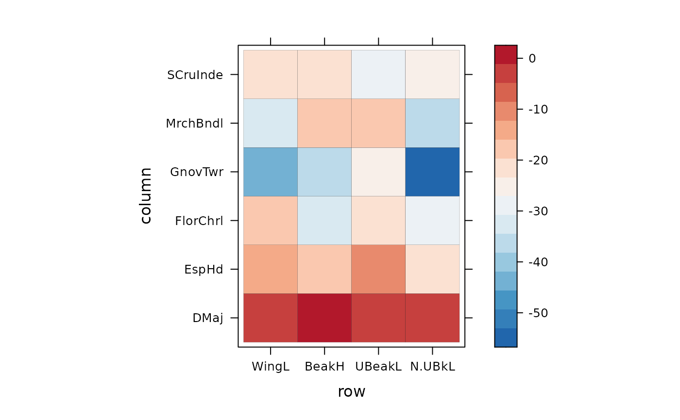
 #### An other way to see "ses values" of T-statistics
# Custom theme (from rasterVis package)
require(rasterVis)
#> Loading required package: rasterVis
#> Loading required package: lattice
my.theme <- BuRdTheme()
# Customize the colorkey
my.ckey <- list(col = my.theme$regions$col)
levelplot(t(ses(res.finch$Tstats$T_IP.IC,res.finch$Tstats$T_IP.IC_nm)$ses),
colorkey = my.ckey, par.settings = my.theme,border = "black")
#### An other way to see "ses values" of T-statistics
# Custom theme (from rasterVis package)
require(rasterVis)
#> Loading required package: rasterVis
#> Loading required package: lattice
my.theme <- BuRdTheme()
# Customize the colorkey
my.ckey <- list(col = my.theme$regions$col)
levelplot(t(ses(res.finch$Tstats$T_IP.IC,res.finch$Tstats$T_IP.IC_nm)$ses),
colorkey = my.ckey, par.settings = my.theme,border = "black")
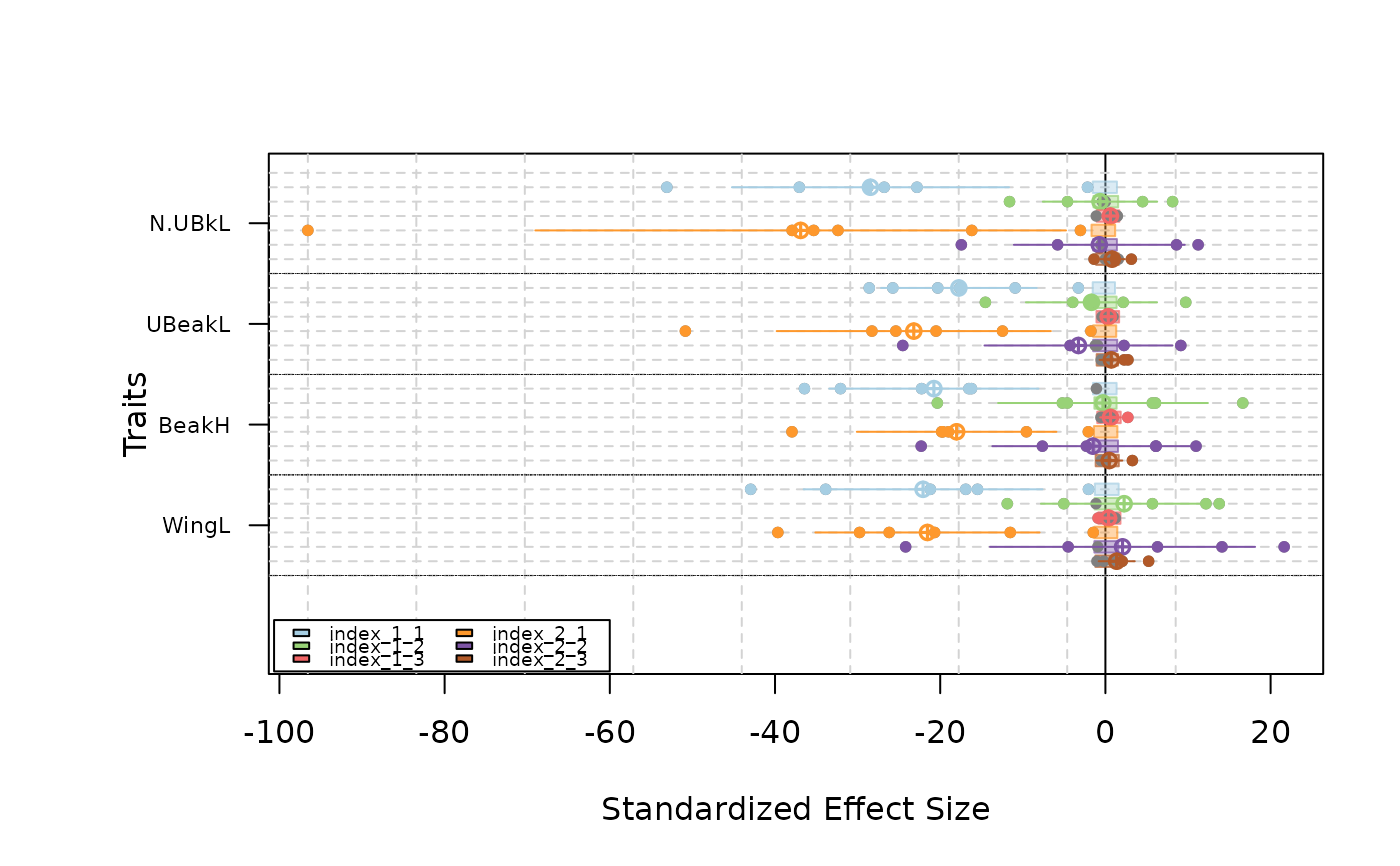
 #### Use a different regional pool than the binding of studied communities
#create a random regional pool for the example
reg.p <- rbind(traits.finch, traits.finch[sample(1:2000,300), ])
res.finch2 <- Tstats(traits.finch, ind.plot = ind.plot.finch,
sp = sp.finch, reg.pool=reg.p, nperm = 9, printprogress = FALSE)
#> Warning: This function exclude 1137 Na values
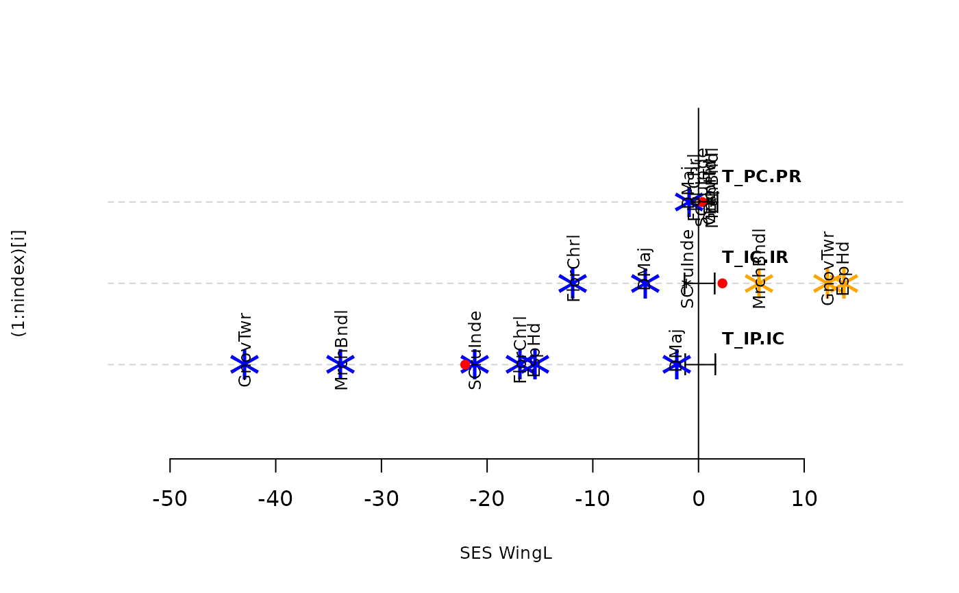
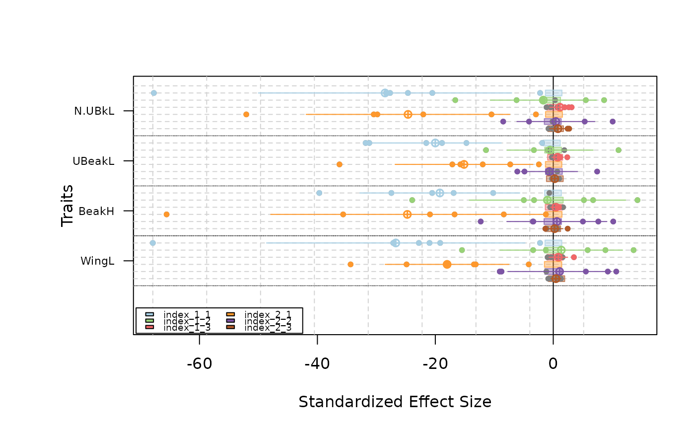
plot(as.listofindex(list(res.finch,res.finch2)))
#### Use a different regional pool than the binding of studied communities
#create a random regional pool for the example
reg.p <- rbind(traits.finch, traits.finch[sample(1:2000,300), ])
res.finch2 <- Tstats(traits.finch, ind.plot = ind.plot.finch,
sp = sp.finch, reg.pool=reg.p, nperm = 9, printprogress = FALSE)
#> Warning: This function exclude 1137 Na values
plot(as.listofindex(list(res.finch,res.finch2)))
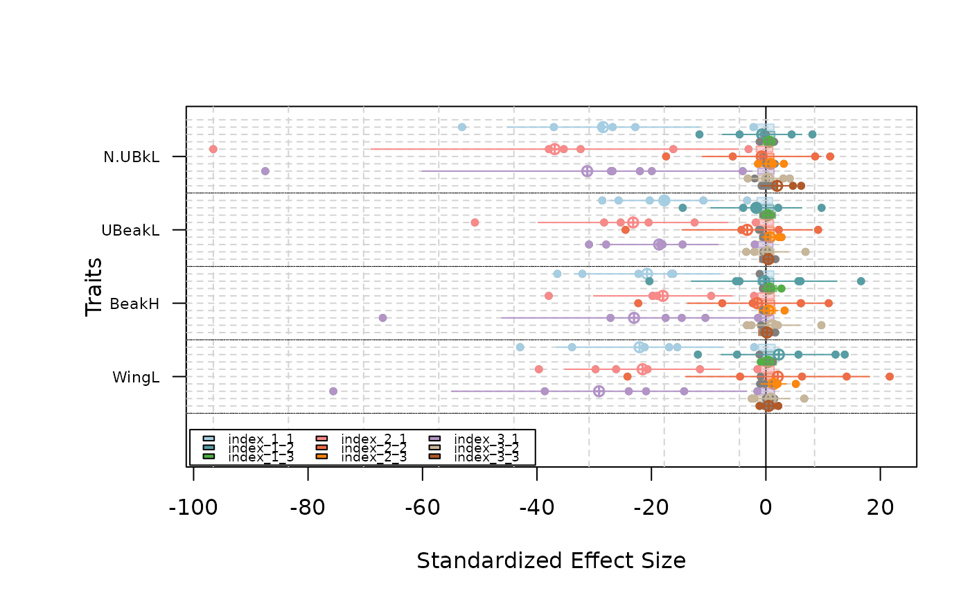
 #### Use a different regional pool for each communities
#create a random regional pool for each communities for the example
list.reg.p <- list(
traits.finch[sample(1:290,200), ], traits.finch[sample(100:1200,300), ],
traits.finch[sample(100:1500, 1000), ], traits.finch[sample(300:800,300), ],
traits.finch[sample(1000:2000, 500), ], traits.finch[sample(100:900, 700), ] )
# Warning: the regional pool need to be larger than the observed communities
table(ind.plot.finch)
#> ind.plot.finch
#> DMaj EspHd FlorChrl GnovTwr MrchBndl SCruInde
#> 50 267 981 258 270 687
# For exemple, the third community need a regional pool of more than 981 individuals
res.finch3 <- Tstats(traits.finch, ind.plot = ind.plot.finch,
sp = sp.finch, reg.pool=list.reg.p, nperm = 9, printprogress = FALSE)
#> Warning: This function exclude 1137 Na values
plot(as.listofindex(list(res.finch, res.finch2, res.finch3)))
#### Use a different regional pool for each communities
#create a random regional pool for each communities for the example
list.reg.p <- list(
traits.finch[sample(1:290,200), ], traits.finch[sample(100:1200,300), ],
traits.finch[sample(100:1500, 1000), ], traits.finch[sample(300:800,300), ],
traits.finch[sample(1000:2000, 500), ], traits.finch[sample(100:900, 700), ] )
# Warning: the regional pool need to be larger than the observed communities
table(ind.plot.finch)
#> ind.plot.finch
#> DMaj EspHd FlorChrl GnovTwr MrchBndl SCruInde
#> 50 267 981 258 270 687
# For exemple, the third community need a regional pool of more than 981 individuals
res.finch3 <- Tstats(traits.finch, ind.plot = ind.plot.finch,
sp = sp.finch, reg.pool=list.reg.p, nperm = 9, printprogress = FALSE)
#> Warning: This function exclude 1137 Na values
plot(as.listofindex(list(res.finch, res.finch2, res.finch3)))
 #### Use the standard errors of measure in the analysis (argument SE)
res.finch.SE0 <- Tstats(traits.finch, ind.plot = ind.plot.finch,
sp = sp.finch, SE = 0, nperm = 9, printprogress = FALSE)
#> Warning: This function exclude 1137 Na values
res.finch.SE5 <- Tstats(traits.finch, ind.plot = ind.plot.finch,
sp = sp.finch, SE = 5, nperm = 9, printprogress = FALSE)
#> Warning: This function exclude 1137 Na values
#> Warning: NAs produced
#> Warning: NAs produced
#> Warning: NAs produced
#> Warning: NAs produced
#> Warning: NAs produced
#> Warning: NAs produced
#> Warning: NAs produced
#> Warning: NAs produced
#> Warning: NAs produced
#> Warning: NAs produced
#> Warning: NAs produced
#> Warning: NAs produced
#> Warning: NAs produced
#> Warning: NAs produced
#> Warning: NAs produced
#> Warning: NAs produced
#> Warning: NAs produced
#> Warning: NAs produced
#> Warning: NAs produced
#> Warning: NAs produced
#> Warning: NAs produced
#> Warning: NAs produced
#> Warning: NAs produced
#> Warning: NAs produced
#> Warning: NAs produced
#> Warning: NAs produced
#> Warning: NAs produced
#> Warning: NAs produced
#> Warning: NAs produced
#> Warning: NAs produced
#> Warning: NAs produced
#> Warning: NAs produced
#> Warning: NAs produced
#> Warning: NAs produced
#> Warning: NAs produced
#> Warning: NAs produced
#> Warning: NAs produced
#> Warning: NAs produced
#> Warning: NAs produced
#> Warning: NAs produced
#> Warning: NAs produced
#> Warning: NAs produced
#> Warning: NAs produced
#> Warning: NAs produced
#> Warning: NAs produced
#> Warning: NAs produced
#> Warning: NAs produced
#> Warning: NAs produced
#> Warning: NAs produced
#> Warning: NAs produced
#> Warning: NAs produced
#> Warning: NAs produced
#> Warning: NAs produced
#> Warning: NAs produced
#> Warning: NAs produced
#> Warning: NAs produced
#> Warning: NAs produced
#> Warning: NAs produced
#> Warning: NAs produced
#> Warning: NAs produced
#> Warning: NAs produced
#> Warning: NAs produced
#> Warning: NAs produced
#> Warning: NAs produced
#> Warning: NAs produced
#> Warning: NAs produced
#> Warning: NAs produced
#> Warning: NAs produced
#> Warning: NAs produced
#> Warning: NAs produced
#> Warning: NAs produced
#> Warning: NAs produced
#> Warning: NAs produced
#> Warning: NAs produced
#> Warning: NAs produced
#> Warning: NAs produced
#> Warning: NAs produced
#> Warning: NAs produced
#> Warning: NAs produced
#> Warning: NAs produced
#> Warning: NAs produced
#> Warning: NAs produced
#> Warning: NAs produced
#> Warning: NAs produced
#> Warning: NAs produced
#> Warning: NAs produced
#> Warning: NAs produced
#> Warning: NAs produced
#> Warning: NAs produced
#> Warning: NAs produced
#> Warning: NAs produced
#> Warning: NAs produced
#> Warning: NAs produced
#> Warning: NAs produced
#> Warning: NAs produced
#> Warning: NAs produced
#> Warning: NAs produced
#> Warning: NAs produced
#> Warning: NAs produced
#> Warning: NAs produced
#> Warning: NAs produced
#> Warning: NAs produced
#> Warning: NAs produced
#> Warning: NAs produced
#> Warning: NAs produced
#> Warning: NAs produced
#> Warning: NAs produced
#> Warning: NAs produced
#> Warning: NAs produced
#> Warning: NAs produced
#> Warning: NAs produced
#> Warning: NAs produced
#> Warning: NAs produced
#> Warning: NAs produced
#> Warning: NAs produced
#> Warning: NAs produced
#> Warning: NAs produced
#> Warning: NAs produced
#> Warning: NAs produced
#> Warning: NAs produced
#> Warning: NAs produced
#> Warning: NAs produced
#> Warning: NAs produced
#> Warning: NAs produced
#> Warning: NAs produced
#> Warning: NAs produced
#> Warning: NAs produced
#> Warning: NAs produced
#> Warning: NAs produced
#> Warning: NAs produced
#> Warning: NAs produced
#> Warning: NAs produced
#> Warning: NAs produced
#> Warning: NAs produced
#> Warning: NAs produced
#> Warning: NAs produced
#> Warning: NAs produced
#> Warning: NAs produced
#> Warning: NAs produced
#> Warning: NAs produced
#> Warning: NAs produced
#> Warning: NAs produced
#> Warning: NAs produced
#> Warning: NAs produced
#> Warning: NAs produced
#> Warning: NAs produced
#> Warning: NAs produced
#> Warning: NAs produced
#> Warning: NAs produced
#> Warning: NAs produced
#> Warning: NAs produced
#> Warning: NAs produced
#> Warning: NAs produced
#> Warning: NAs produced
#> Warning: NAs produced
#> Warning: NAs produced
#> Warning: NAs produced
#> Warning: NAs produced
#> Warning: NAs produced
#> Warning: NAs produced
#> Warning: NAs produced
#> Warning: NAs produced
#> Warning: NAs produced
#> Warning: NAs produced
#> Warning: NAs produced
#> Warning: NAs produced
#> Warning: NAs produced
#> Warning: NAs produced
#> Warning: NAs produced
#> Warning: NAs produced
#> Warning: NAs produced
#> Warning: NAs produced
#> Warning: NAs produced
#> Warning: NAs produced
#> Warning: NAs produced
#> Warning: NAs produced
#> Warning: NAs produced
#> Warning: NAs produced
#> Warning: NAs produced
#> Warning: NAs produced
#> Warning: NAs produced
#> Warning: NAs produced
#> Warning: NAs produced
#> Warning: NAs produced
#> Warning: NAs produced
#> Warning: NAs produced
#> Warning: NAs produced
#> Warning: NAs produced
#> Warning: NAs produced
#> Warning: NAs produced
#> Warning: NAs produced
#> Warning: NAs produced
#> Warning: NAs produced
#> Warning: NAs produced
#> Warning: NAs produced
#> Warning: NAs produced
#> Warning: NAs produced
#> Warning: NAs produced
#> Warning: NAs produced
#> Warning: NAs produced
#> Warning: NAs produced
#> Warning: NAs produced
#> Warning: NAs produced
#> Warning: NAs produced
#> Warning: NAs produced
#> Warning: NAs produced
#> Warning: NAs produced
#> Warning: NAs produced
#> Warning: NAs produced
#> Warning: NAs produced
#> Warning: NAs produced
#> Warning: NAs produced
#> Warning: NAs produced
#> Warning: NAs produced
#> Warning: NAs produced
#> Warning: NAs produced
#> Warning: NAs produced
#> Warning: NAs produced
#> Warning: NAs produced
#> Warning: NAs produced
#> Warning: NAs produced
#> Warning: NAs produced
#> Warning: NAs produced
#> Warning: NAs produced
#> Warning: NAs produced
#> Warning: NAs produced
#> Warning: NAs produced
#> Warning: NAs produced
#> Warning: NAs produced
#> Warning: NAs produced
#> Warning: NAs produced
#> Warning: NAs produced
#> Warning: NAs produced
#> Warning: NAs produced
#> Warning: NAs produced
#> Warning: NAs produced
#> Warning: NAs produced
#> Warning: NAs produced
#> Warning: NAs produced
#> Warning: NAs produced
#> Warning: NAs produced
#> Warning: NAs produced
#> Warning: NAs produced
#> Warning: NAs produced
#> Warning: NAs produced
#> Warning: NAs produced
#> Warning: NAs produced
#> Warning: NAs produced
#> Warning: NAs produced
#> Warning: NAs produced
#> Warning: NAs produced
#> Warning: NAs produced
#> Warning: NAs produced
#> Warning: NAs produced
#> Warning: NAs produced
#> Warning: NAs produced
#> Warning: NAs produced
#> Warning: NAs produced
#> Warning: NAs produced
#> Warning: NAs produced
#> Warning: NAs produced
#> Warning: NAs produced
#> Warning: NAs produced
#> Warning: NAs produced
#> Warning: NAs produced
#> Warning: NAs produced
#> Warning: NAs produced
#> Warning: NAs produced
#> Warning: NAs produced
#> Warning: NAs produced
#> Warning: NAs produced
#> Warning: NAs produced
#> Warning: NAs produced
#> Warning: NAs produced
#> Warning: NAs produced
#> Warning: NAs produced
#> Warning: NAs produced
#> Warning: NAs produced
#> Warning: NAs produced
#> Warning: NAs produced
#> Warning: NAs produced
#> Warning: NAs produced
#> Warning: NAs produced
#> Warning: NAs produced
#> Warning: NAs produced
#> Warning: NAs produced
#> Warning: NAs produced
#> Warning: NAs produced
#> Warning: NAs produced
#> Warning: NAs produced
#> Warning: NAs produced
#> Warning: NAs produced
#> Warning: NAs produced
#> Warning: NAs produced
#> Warning: NAs produced
#> Warning: NAs produced
#> Warning: NAs produced
#> Warning: NAs produced
#> Warning: NAs produced
#> Warning: NAs produced
#> Warning: NAs produced
#> Warning: NAs produced
#> Warning: NAs produced
#> Warning: NAs produced
#> Warning: NAs produced
#> Warning: NAs produced
#> Warning: NAs produced
#> Warning: NAs produced
#> Warning: NAs produced
#> Warning: NAs produced
#> Warning: NAs produced
#> Warning: NAs produced
#> Warning: NAs produced
#> Warning: NAs produced
#> Warning: NAs produced
#> Warning: NAs produced
#> Warning: NAs produced
#> Warning: NAs produced
#> Warning: NAs produced
#> Warning: NAs produced
#> Warning: NAs produced
#> Warning: NAs produced
#> Warning: NAs produced
#> Warning: NAs produced
#> Warning: NAs produced
#> Warning: NAs produced
#> Warning: NAs produced
#> Warning: NAs produced
#> Warning: NAs produced
#> Warning: NAs produced
#> Warning: NAs produced
#> Warning: NAs produced
#> Warning: NAs produced
#> Warning: NAs produced
#> Warning: NAs produced
#> Warning: NAs produced
#> Warning: NAs produced
#> Warning: NAs produced
#> Warning: NAs produced
#> Warning: NAs produced
#> Warning: NAs produced
#> Warning: NAs produced
#> Warning: NAs produced
#> Warning: NAs produced
#> Warning: NAs produced
#> Warning: NAs produced
#> Warning: NAs produced
#> Warning: NAs produced
#> Warning: NAs produced
#> Warning: NAs produced
#> Warning: NAs produced
#> Warning: NAs produced
#> Warning: NAs produced
#> Warning: NAs produced
#> Warning: NAs produced
#> Warning: NAs produced
#> Warning: NAs produced
#> Warning: NAs produced
#> Warning: NAs produced
#> Warning: NAs produced
#> Warning: NAs produced
#> Warning: NAs produced
#> Warning: NAs produced
#> Warning: NAs produced
#> Warning: NAs produced
#> Warning: NAs produced
#> Warning: NAs produced
#> Warning: NAs produced
#> Warning: NAs produced
#> Warning: NAs produced
#> Warning: NAs produced
#> Warning: NAs produced
#> Warning: NAs produced
#> Warning: NAs produced
#> Warning: NAs produced
#> Warning: NAs produced
#> Warning: NAs produced
#> Warning: NAs produced
#> Warning: NAs produced
#> Warning: NAs produced
#> Warning: NAs produced
#> Warning: NAs produced
#> Warning: NAs produced
#> Warning: NAs produced
#> Warning: NAs produced
#> Warning: NAs produced
#> Warning: NAs produced
#> Warning: NAs produced
#> Warning: NAs produced
#> Warning: NAs produced
#> Warning: NAs produced
#> Warning: NAs produced
#> Warning: NAs produced
#> Warning: NAs produced
#> Warning: NAs produced
#> Warning: NAs produced
#> Warning: NAs produced
#> Warning: NAs produced
#> Warning: NAs produced
#> Warning: NAs produced
#> Warning: NAs produced
#> Warning: NAs produced
#> Warning: NAs produced
#> Warning: NAs produced
#> Warning: NAs produced
#> Warning: NAs produced
#> Warning: NAs produced
#> Warning: NAs produced
#> Warning: NAs produced
#> Warning: NAs produced
#> Warning: NAs produced
#> Warning: NAs produced
#> Warning: NAs produced
#> Warning: NAs produced
#> Warning: NAs produced
#> Warning: NAs produced
#> Warning: NAs produced
#> Warning: NAs produced
#> Warning: NAs produced
#> Warning: NAs produced
#> Warning: NAs produced
#> Warning: NAs produced
#> Warning: NAs produced
#> Warning: NAs produced
#> Warning: NAs produced
#> Warning: NAs produced
#> Warning: NAs produced
#> Warning: NAs produced
#> Warning: NAs produced
#> Warning: NAs produced
#> Warning: NAs produced
#> Warning: NAs produced
plot(as.listofindex(list(res.finch.SE0, res.finch.SE5)))
#### Use the standard errors of measure in the analysis (argument SE)
res.finch.SE0 <- Tstats(traits.finch, ind.plot = ind.plot.finch,
sp = sp.finch, SE = 0, nperm = 9, printprogress = FALSE)
#> Warning: This function exclude 1137 Na values
res.finch.SE5 <- Tstats(traits.finch, ind.plot = ind.plot.finch,
sp = sp.finch, SE = 5, nperm = 9, printprogress = FALSE)
#> Warning: This function exclude 1137 Na values
#> Warning: NAs produced
#> Warning: NAs produced
#> Warning: NAs produced
#> Warning: NAs produced
#> Warning: NAs produced
#> Warning: NAs produced
#> Warning: NAs produced
#> Warning: NAs produced
#> Warning: NAs produced
#> Warning: NAs produced
#> Warning: NAs produced
#> Warning: NAs produced
#> Warning: NAs produced
#> Warning: NAs produced
#> Warning: NAs produced
#> Warning: NAs produced
#> Warning: NAs produced
#> Warning: NAs produced
#> Warning: NAs produced
#> Warning: NAs produced
#> Warning: NAs produced
#> Warning: NAs produced
#> Warning: NAs produced
#> Warning: NAs produced
#> Warning: NAs produced
#> Warning: NAs produced
#> Warning: NAs produced
#> Warning: NAs produced
#> Warning: NAs produced
#> Warning: NAs produced
#> Warning: NAs produced
#> Warning: NAs produced
#> Warning: NAs produced
#> Warning: NAs produced
#> Warning: NAs produced
#> Warning: NAs produced
#> Warning: NAs produced
#> Warning: NAs produced
#> Warning: NAs produced
#> Warning: NAs produced
#> Warning: NAs produced
#> Warning: NAs produced
#> Warning: NAs produced
#> Warning: NAs produced
#> Warning: NAs produced
#> Warning: NAs produced
#> Warning: NAs produced
#> Warning: NAs produced
#> Warning: NAs produced
#> Warning: NAs produced
#> Warning: NAs produced
#> Warning: NAs produced
#> Warning: NAs produced
#> Warning: NAs produced
#> Warning: NAs produced
#> Warning: NAs produced
#> Warning: NAs produced
#> Warning: NAs produced
#> Warning: NAs produced
#> Warning: NAs produced
#> Warning: NAs produced
#> Warning: NAs produced
#> Warning: NAs produced
#> Warning: NAs produced
#> Warning: NAs produced
#> Warning: NAs produced
#> Warning: NAs produced
#> Warning: NAs produced
#> Warning: NAs produced
#> Warning: NAs produced
#> Warning: NAs produced
#> Warning: NAs produced
#> Warning: NAs produced
#> Warning: NAs produced
#> Warning: NAs produced
#> Warning: NAs produced
#> Warning: NAs produced
#> Warning: NAs produced
#> Warning: NAs produced
#> Warning: NAs produced
#> Warning: NAs produced
#> Warning: NAs produced
#> Warning: NAs produced
#> Warning: NAs produced
#> Warning: NAs produced
#> Warning: NAs produced
#> Warning: NAs produced
#> Warning: NAs produced
#> Warning: NAs produced
#> Warning: NAs produced
#> Warning: NAs produced
#> Warning: NAs produced
#> Warning: NAs produced
#> Warning: NAs produced
#> Warning: NAs produced
#> Warning: NAs produced
#> Warning: NAs produced
#> Warning: NAs produced
#> Warning: NAs produced
#> Warning: NAs produced
#> Warning: NAs produced
#> Warning: NAs produced
#> Warning: NAs produced
#> Warning: NAs produced
#> Warning: NAs produced
#> Warning: NAs produced
#> Warning: NAs produced
#> Warning: NAs produced
#> Warning: NAs produced
#> Warning: NAs produced
#> Warning: NAs produced
#> Warning: NAs produced
#> Warning: NAs produced
#> Warning: NAs produced
#> Warning: NAs produced
#> Warning: NAs produced
#> Warning: NAs produced
#> Warning: NAs produced
#> Warning: NAs produced
#> Warning: NAs produced
#> Warning: NAs produced
#> Warning: NAs produced
#> Warning: NAs produced
#> Warning: NAs produced
#> Warning: NAs produced
#> Warning: NAs produced
#> Warning: NAs produced
#> Warning: NAs produced
#> Warning: NAs produced
#> Warning: NAs produced
#> Warning: NAs produced
#> Warning: NAs produced
#> Warning: NAs produced
#> Warning: NAs produced
#> Warning: NAs produced
#> Warning: NAs produced
#> Warning: NAs produced
#> Warning: NAs produced
#> Warning: NAs produced
#> Warning: NAs produced
#> Warning: NAs produced
#> Warning: NAs produced
#> Warning: NAs produced
#> Warning: NAs produced
#> Warning: NAs produced
#> Warning: NAs produced
#> Warning: NAs produced
#> Warning: NAs produced
#> Warning: NAs produced
#> Warning: NAs produced
#> Warning: NAs produced
#> Warning: NAs produced
#> Warning: NAs produced
#> Warning: NAs produced
#> Warning: NAs produced
#> Warning: NAs produced
#> Warning: NAs produced
#> Warning: NAs produced
#> Warning: NAs produced
#> Warning: NAs produced
#> Warning: NAs produced
#> Warning: NAs produced
#> Warning: NAs produced
#> Warning: NAs produced
#> Warning: NAs produced
#> Warning: NAs produced
#> Warning: NAs produced
#> Warning: NAs produced
#> Warning: NAs produced
#> Warning: NAs produced
#> Warning: NAs produced
#> Warning: NAs produced
#> Warning: NAs produced
#> Warning: NAs produced
#> Warning: NAs produced
#> Warning: NAs produced
#> Warning: NAs produced
#> Warning: NAs produced
#> Warning: NAs produced
#> Warning: NAs produced
#> Warning: NAs produced
#> Warning: NAs produced
#> Warning: NAs produced
#> Warning: NAs produced
#> Warning: NAs produced
#> Warning: NAs produced
#> Warning: NAs produced
#> Warning: NAs produced
#> Warning: NAs produced
#> Warning: NAs produced
#> Warning: NAs produced
#> Warning: NAs produced
#> Warning: NAs produced
#> Warning: NAs produced
#> Warning: NAs produced
#> Warning: NAs produced
#> Warning: NAs produced
#> Warning: NAs produced
#> Warning: NAs produced
#> Warning: NAs produced
#> Warning: NAs produced
#> Warning: NAs produced
#> Warning: NAs produced
#> Warning: NAs produced
#> Warning: NAs produced
#> Warning: NAs produced
#> Warning: NAs produced
#> Warning: NAs produced
#> Warning: NAs produced
#> Warning: NAs produced
#> Warning: NAs produced
#> Warning: NAs produced
#> Warning: NAs produced
#> Warning: NAs produced
#> Warning: NAs produced
#> Warning: NAs produced
#> Warning: NAs produced
#> Warning: NAs produced
#> Warning: NAs produced
#> Warning: NAs produced
#> Warning: NAs produced
#> Warning: NAs produced
#> Warning: NAs produced
#> Warning: NAs produced
#> Warning: NAs produced
#> Warning: NAs produced
#> Warning: NAs produced
#> Warning: NAs produced
#> Warning: NAs produced
#> Warning: NAs produced
#> Warning: NAs produced
#> Warning: NAs produced
#> Warning: NAs produced
#> Warning: NAs produced
#> Warning: NAs produced
#> Warning: NAs produced
#> Warning: NAs produced
#> Warning: NAs produced
#> Warning: NAs produced
#> Warning: NAs produced
#> Warning: NAs produced
#> Warning: NAs produced
#> Warning: NAs produced
#> Warning: NAs produced
#> Warning: NAs produced
#> Warning: NAs produced
#> Warning: NAs produced
#> Warning: NAs produced
#> Warning: NAs produced
#> Warning: NAs produced
#> Warning: NAs produced
#> Warning: NAs produced
#> Warning: NAs produced
#> Warning: NAs produced
#> Warning: NAs produced
#> Warning: NAs produced
#> Warning: NAs produced
#> Warning: NAs produced
#> Warning: NAs produced
#> Warning: NAs produced
#> Warning: NAs produced
#> Warning: NAs produced
#> Warning: NAs produced
#> Warning: NAs produced
#> Warning: NAs produced
#> Warning: NAs produced
#> Warning: NAs produced
#> Warning: NAs produced
#> Warning: NAs produced
#> Warning: NAs produced
#> Warning: NAs produced
#> Warning: NAs produced
#> Warning: NAs produced
#> Warning: NAs produced
#> Warning: NAs produced
#> Warning: NAs produced
#> Warning: NAs produced
#> Warning: NAs produced
#> Warning: NAs produced
#> Warning: NAs produced
#> Warning: NAs produced
#> Warning: NAs produced
#> Warning: NAs produced
#> Warning: NAs produced
#> Warning: NAs produced
#> Warning: NAs produced
#> Warning: NAs produced
#> Warning: NAs produced
#> Warning: NAs produced
#> Warning: NAs produced
#> Warning: NAs produced
#> Warning: NAs produced
#> Warning: NAs produced
#> Warning: NAs produced
#> Warning: NAs produced
#> Warning: NAs produced
#> Warning: NAs produced
#> Warning: NAs produced
#> Warning: NAs produced
#> Warning: NAs produced
#> Warning: NAs produced
#> Warning: NAs produced
#> Warning: NAs produced
#> Warning: NAs produced
#> Warning: NAs produced
#> Warning: NAs produced
#> Warning: NAs produced
#> Warning: NAs produced
#> Warning: NAs produced
#> Warning: NAs produced
#> Warning: NAs produced
#> Warning: NAs produced
#> Warning: NAs produced
#> Warning: NAs produced
#> Warning: NAs produced
#> Warning: NAs produced
#> Warning: NAs produced
#> Warning: NAs produced
#> Warning: NAs produced
#> Warning: NAs produced
#> Warning: NAs produced
#> Warning: NAs produced
#> Warning: NAs produced
#> Warning: NAs produced
#> Warning: NAs produced
#> Warning: NAs produced
#> Warning: NAs produced
#> Warning: NAs produced
#> Warning: NAs produced
#> Warning: NAs produced
#> Warning: NAs produced
#> Warning: NAs produced
#> Warning: NAs produced
#> Warning: NAs produced
#> Warning: NAs produced
#> Warning: NAs produced
#> Warning: NAs produced
#> Warning: NAs produced
#> Warning: NAs produced
#> Warning: NAs produced
#> Warning: NAs produced
#> Warning: NAs produced
#> Warning: NAs produced
#> Warning: NAs produced
#> Warning: NAs produced
#> Warning: NAs produced
#> Warning: NAs produced
#> Warning: NAs produced
#> Warning: NAs produced
#> Warning: NAs produced
#> Warning: NAs produced
#> Warning: NAs produced
#> Warning: NAs produced
#> Warning: NAs produced
#> Warning: NAs produced
#> Warning: NAs produced
#> Warning: NAs produced
#> Warning: NAs produced
#> Warning: NAs produced
#> Warning: NAs produced
#> Warning: NAs produced
#> Warning: NAs produced
#> Warning: NAs produced
#> Warning: NAs produced
#> Warning: NAs produced
#> Warning: NAs produced
#> Warning: NAs produced
#> Warning: NAs produced
#> Warning: NAs produced
#> Warning: NAs produced
#> Warning: NAs produced
#> Warning: NAs produced
#> Warning: NAs produced
#> Warning: NAs produced
#> Warning: NAs produced
#> Warning: NAs produced
#> Warning: NAs produced
#> Warning: NAs produced
#> Warning: NAs produced
#> Warning: NAs produced
#> Warning: NAs produced
#> Warning: NAs produced
#> Warning: NAs produced
#> Warning: NAs produced
#> Warning: NAs produced
#> Warning: NAs produced
#> Warning: NAs produced
#> Warning: NAs produced
#> Warning: NAs produced
#> Warning: NAs produced
#> Warning: NAs produced
#> Warning: NAs produced
#> Warning: NAs produced
#> Warning: NAs produced
#> Warning: NAs produced
#> Warning: NAs produced
#> Warning: NAs produced
#> Warning: NAs produced
#> Warning: NAs produced
#> Warning: NAs produced
#> Warning: NAs produced
#> Warning: NAs produced
#> Warning: NAs produced
#> Warning: NAs produced
#> Warning: NAs produced
#> Warning: NAs produced
#> Warning: NAs produced
#> Warning: NAs produced
#> Warning: NAs produced
#> Warning: NAs produced
#> Warning: NAs produced
#> Warning: NAs produced
#> Warning: NAs produced
#> Warning: NAs produced
#> Warning: NAs produced
#> Warning: NAs produced
#> Warning: NAs produced
#> Warning: NAs produced
#> Warning: NAs produced
#> Warning: NAs produced
#> Warning: NAs produced
#> Warning: NAs produced
#> Warning: NAs produced
#> Warning: NAs produced
#> Warning: NAs produced
#> Warning: NAs produced
#> Warning: NAs produced
#> Warning: NAs produced
#> Warning: NAs produced
#> Warning: NAs produced
#> Warning: NAs produced
#> Warning: NAs produced
plot(as.listofindex(list(res.finch.SE0, res.finch.SE5)))
 # }
# }