Benchmarking Differential Abundance Methods

Introduction

This vignette provides a comprehensive benchmark of differential abundance (DA) methods for microbiome data, inspired by the benchdamic package approach. We compare seven methods:

Method	Package	Approach
ALDEx2	ALDEx2	CLR transformation + Monte Carlo sampling from Dirichlet
ANCOM-BC2	ANCOMBC	Linear regression with bias correction
MaAsLin3	maaslin3	Generalized linear models (abundance + prevalence)
DESeq2	DESeq2	Negative binomial GLM with size factor normalization
edgeR	edgeR	Negative binomial GLM with TMM normalization
limma-voom	limma	Linear models on voom-transformed counts
radEmu	radEmu	Robust estimation for relative abundance data

The benchmark evaluates:

Method concordance: Agreement between methods on significant taxa
Effect size correlation: Consistency of effect size estimates
Sensitivity/Specificity trade-off: Using simulated spike-in data
Computational considerations: Runtime and ease of use

Setup

library(comparpq)
library(phyloseq)
library(ggplot2)
library(dplyr)
library(tidyr)
library(tibble)
library(patchwork)

# For DA methods
library(DESeq2)
library(edgeR)
library(limma)
library(radEmu)
library(ALDEx2)
library(BiocParallel)

Helper Functions

We define wrapper functions to standardize output across methods.

#' Run DESeq2 on phyloseq object
#' @param physeq A phyloseq object
#' @param formula Formula for the design (e.g., "~ condition")
#' @param contrast Character vector for contrast (e.g., c("condition", "B", "A"))
#' @param nclusters Number of cores for parallel processing (default 1)
#' @return Data frame with taxon, effect (log2FC), pvalue, qvalue
run_deseq2 <- function(physeq, formula, contrast, nclusters = 1) {
  # Convert to DESeq2
  dds <- phyloseq_to_deseq2(physeq, as.formula(formula))

  # Set up parallel processing
  if (nclusters > 1) {
    BPPARAM <- BiocParallel::MulticoreParam(workers = nclusters)
  } else {
    BPPARAM <- BiocParallel::SerialParam()
  }

  # Run DESeq2 with geometric mean estimation that handles zeros
  dds <- DESeq2::estimateSizeFactors(dds, type = "poscounts")
  dds <- DESeq2::estimateDispersions(dds, fitType = "local")
  dds <- DESeq2::nbinomWaldTest(dds)

  # Get results
  res <- DESeq2::results(dds, contrast = contrast, parallel = nclusters > 1, BPPARAM = BPPARAM)

  data.frame(
    taxon = rownames(res),
    effect = res$log2FoldChange,
    pvalue = res$pvalue,
    qvalue = res$padj,
    method = "DESeq2",
    stringsAsFactors = FALSE
  ) |>
    filter(!is.na(effect))
}

#' Run edgeR on phyloseq object
#' @param physeq A phyloseq object
#' @param group_var Name of grouping variable in sample_data
#' @param contrast_levels Two-element vector: c(treatment, reference)
#' @return Data frame with taxon, effect (logFC), pvalue, qvalue
run_edgeR <- function(physeq, group_var, contrast_levels) {
  # Extract data
  counts <- as(otu_table(physeq), "matrix")
  if (!taxa_are_rows(physeq)) counts <- t(counts)

  group <- factor(sample_data(physeq)[[group_var]])
  group <- relevel(group, ref = contrast_levels[2])

  # Create DGEList
  dge <- edgeR::DGEList(counts = counts, group = group)

  # Filter low counts
  keep <- edgeR::filterByExpr(dge)
  dge <- dge[keep, , keep.lib.sizes = FALSE]

  # Normalize
  dge <- edgeR::calcNormFactors(dge, method = "TMM")

  # Design matrix
  design <- model.matrix(~ group)

 # Estimate dispersion
  dge <- edgeR::estimateDisp(dge, design)

  # Fit model
  fit <- edgeR::glmQLFit(dge, design)
  qlf <- edgeR::glmQLFTest(fit, coef = 2)

  # Get results
  res <- edgeR::topTags(qlf, n = Inf)$table

  data.frame(
    taxon = rownames(res),
    effect = res$logFC,
    pvalue = res$PValue,
    qvalue = res$FDR,
    method = "edgeR",
    stringsAsFactors = FALSE
  )
}

#' Run limma-voom on phyloseq object
#' @param physeq A phyloseq object
#' @param group_var Name of grouping variable in sample_data
#' @param contrast_levels Two-element vector: c(treatment, reference)
#' @return Data frame with taxon, effect (logFC), pvalue, qvalue
run_limma_voom <- function(physeq, group_var, contrast_levels) {
  # Extract data
  counts <- as(otu_table(physeq), "matrix")
  if (!taxa_are_rows(physeq)) counts <- t(counts)

  group <- factor(sample_data(physeq)[[group_var]])
  group <- relevel(group, ref = contrast_levels[2])

  # Create DGEList for normalization
  dge <- edgeR::DGEList(counts = counts, group = group)

  # Filter low counts
  keep <- edgeR::filterByExpr(dge)
  dge <- dge[keep, , keep.lib.sizes = FALSE]

  # Normalize
  dge <- edgeR::calcNormFactors(dge, method = "TMM")

  # Design matrix
  design <- model.matrix(~ group)

  # Voom transformation
  v <- limma::voom(dge, design, plot = FALSE)

  # Fit linear model
  fit <- limma::lmFit(v, design)
  fit <- limma::eBayes(fit)

  # Get results
  res <- limma::topTable(fit, coef = 2, number = Inf, sort.by = "none")

  data.frame(
    taxon = rownames(res),
    effect = res$logFC,
    pvalue = res$P.Value,
    qvalue = res$adj.P.Val,
    method = "limma-voom",
    stringsAsFactors = FALSE
  )
}

#' Run ALDEx2 on phyloseq object
#' @param physeq A phyloseq object
#' @param group_var Name of grouping variable in sample_data
#' @param contrast_levels Two-element vector: c(treatment, reference)
#' @param nclusters Number of cores for parallel processing (default 1)
#' @return Data frame with taxon, effect, pvalue, qvalue
run_aldex2 <- function(physeq, group_var, contrast_levels, nclusters = 1) {

  # Convert factor to character to avoid ALDEx2 error
  sample_data(physeq)[[group_var]] <- as.character(sample_data(physeq)[[group_var]])

  # Extract counts and conditions for direct ALDEx2 call
  counts <- as(otu_table(physeq), "matrix")
  if (!taxa_are_rows(physeq)) counts <- t(counts)

  conds <- sample_data(physeq)[[group_var]]

  # Run ALDEx2 with parallel support
  clr <- ALDEx2::aldex.clr(
    counts,
    conds,
    mc.samples = 128,
    useMC = nclusters > 1
  )
  tt <- ALDEx2::aldex.ttest(clr)
  effect <- ALDEx2::aldex.effect(clr, useMC = nclusters > 1)
  res <- cbind(tt, effect)

  data.frame(
    taxon = rownames(res),
    effect = res$effect,
    pvalue = res$wi.ep,
    qvalue = res$wi.eBH,
    method = "ALDEx2",
    stringsAsFactors = FALSE
  )
}

#' Run ANCOM-BC2 on phyloseq object
#' @param physeq A phyloseq object
#' @param group_var Name of grouping variable in sample_data
#' @param contrast_levels Two-element vector: c(treatment, reference)
#' @param nclusters Number of cores for parallel processing (default 1)
#' @return Data frame with taxon, effect (lfc), pvalue, qvalue
run_ancombc <- function(physeq, group_var, contrast_levels, nclusters = 1) {
  res <- MiscMetabar::ancombc_pq(
    physeq,
    fact = group_var,
    levels_fact = contrast_levels,
    tax_level = NULL,
    n_cl = nclusters
  )

  # Find the correct column names (depends on factor levels)
  lfc_col <- grep("^lfc_", colnames(res$res), value = TRUE)[1]
  p_col <- grep("^p_", colnames(res$res), value = TRUE)[1]
  q_col <- grep("^q_", colnames(res$res), value = TRUE)[1]

  data.frame(
    taxon = res$res$taxon,
    effect = res$res[[lfc_col]],
    pvalue = res$res[[p_col]],
    qvalue = res$res[[q_col]],
    method = "ANCOM-BC2",
    stringsAsFactors = FALSE
  ) |>
    filter(!is.na(effect))
}

#' Run MaAsLin3 on phyloseq object
#' @param physeq A phyloseq object
#' @param group_var Name of grouping variable in sample_data
#' @param contrast_levels Two-element vector: c(treatment, reference)
#' @param nclusters Number of cores for parallel processing (default 1)
#' @return Data frame with taxon, effect (coef), pvalue, qvalue
run_maaslin3 <- function(physeq, group_var, contrast_levels, nclusters = 1) {
  res <- maaslin3_pq(
    physeq,
    formula = paste0("~ ", group_var),
    reference = setNames(list(contrast_levels[2]), group_var),
    output = tempfile(),
    correction_for_sample_size = TRUE,
    plot_summary_plot = FALSE,
    plot_associations = FALSE,
    cores = nclusters
  )

  df <- res$fit_data_abundance$results |>
    filter(grepl(group_var, metadata))

  data.frame(
    taxon = df$feature,
    effect = df$coef,
    pvalue = df$pval_individual,
    qvalue = df$qval_individual,
    method = "MaAsLin3",
    stringsAsFactors = FALSE
  ) |>
    filter(!is.na(effect))
}

#' Run radEmu on phyloseq object
#' @param physeq A phyloseq object
#' @param group_var Name of grouping variable in sample_data
#' @param contrast_levels Two-element vector: c(treatment, reference)
#' @param return_wald_p If TRUE (default), use fast Wald p-values. If FALSE,
#'   use slower but more robust score tests with two-step filtering.
#' @param effect_threshold Minimum absolute effect to test with score tests
#'   (only used when return_wald_p = FALSE, default 0.5)
#' @param max_taxa_to_test Maximum number of taxa to test with score tests
#'   (only used when return_wald_p = FALSE, default NULL = all)
#' @param nclusters Number of cores for parallel processing (default 1)
#' @param ... Additional arguments passed to `radEmu::emuFit()`
#' @return Data frame with taxon, effect (estimate), pvalue, qvalue
run_emuFit <- function(physeq, 
group_var, 
contrast_levels,
                       return_wald_p = TRUE,
                       effect_threshold = 0.5,
                        max_taxa_to_test = NULL,
                       nclusters = 1, ...) {
  # Remove samples with zero total counts (radEmu requirement)
  sample_totals <- sample_sums(physeq)
  physeq <- prune_samples(sample_totals > 0, physeq)

  # Relevel factor so reference is first
  sample_data(physeq)[[group_var]] <- factor(
    sample_data(physeq)[[group_var]],
    levels = c(contrast_levels[2], contrast_levels[1])
  )

  if (return_wald_p) {
    # Fast approach: single fit with Wald p-values
    fit <- radEmu::emuFit(
      formula = as.formula(paste0("~ ", group_var)),
      Y = physeq,
      run_score_tests = FALSE,
      return_wald_p=return_wald_p,
      ...
    )

    # Extract results (Wald p-values are in pval column)
    coef_df <- fit$coef |>
      filter(covariate != "(Intercept)")

    # Adjust p-values for multiple testing
    coef_df$wald_q <- p.adjust(coef_df$wald_p, method = "BH")

    return(data.frame(
      taxon = coef_df$category,
      effect = coef_df$estimate,
      pvalue = coef_df$wald_p,
      qvalue = coef_df$wald_q,
      method = "radEmu_wald",
      stringsAsFactors = FALSE
    ) |>
      filter(!is.na(effect)))
  }

 # Two-step approach with score tests (slower but more robust)

  # Step 1: Run emuFit WITHOUT testing (fast) to get effect estimates
  fit_effects <- radEmu::emuFit(
    formula = as.formula(paste0("~ ", group_var)),
    Y = physeq,
    run_score_tests = FALSE,
    ...
  )

  # Extract effect estimates
  coef_df <- fit_effects$coef
  coef_df$abs_effect <- abs(coef_df$estimate)

  # Step 2: Select taxa with high effects to test
  # Filter by threshold and optionally limit to max_taxa_to_test
  taxa_to_test <- coef_df |>
    filter(covariate != "(Intercept)", abs_effect >= effect_threshold) |>
    arrange(desc(abs_effect))

  if (!is.null(max_taxa_to_test) && max_taxa_to_test > 0) {
    taxa_to_test <- head(taxa_to_test, max_taxa_to_test)
  }

  if (nrow(taxa_to_test) == 0) {
    # No taxa meet threshold - return all with NA p-values
    return(data.frame(
      taxon = coef_df$category[coef_df$covariate != "(Intercept)"],
      effect = coef_df$estimate[coef_df$covariate != "(Intercept)"],
      pvalue = NA_real_,
      qvalue = NA_real_,
      method = "radEmu",
      stringsAsFactors = FALSE
    ))
  }

  # Get indices of taxa to test (j values)
  taxa_names_vec <- taxa_names(physeq)
  j_to_test <- match(taxa_to_test$category, taxa_names_vec)

  # Step 3: Run emuFit WITH score testing only for selected taxa
  fit_tested <- radEmu::emuFit(
    formula = as.formula(paste0("~ ", group_var)),
    Y = physeq,
    test_kj = data.frame(k = 2, j = j_to_test),
    parallel = nclusters > 1,
    ncores = nclusters
  )

  # Extract tested results
  tested_res <- fit_tested$coef |>
    filter(covariate != "(Intercept)")

  # Merge with all effects
  all_effects <- coef_df |>
    filter(covariate != "(Intercept)") |>
    dplyr::select(category, estimate)

  res <- all_effects |>
    left_join(
      tested_res |> dplyr::select(category, pval),
      by = "category"
    )

  # Adjust p-values for multiple testing (only for tested taxa)
  res$qvalue <- p.adjust(res$pval, method = "BH")

  data.frame(
    taxon = res$category,
    effect = res$estimate,
    pvalue = res$pval,
    qvalue = res$qvalue,
    method = "radEmu_score",
    stringsAsFactors = FALSE
  ) |>
    filter(!is.na(effect))
}

#' Run all DA methods on a phyloseq object
#' @param physeq A phyloseq object
#' @param group_var Name of grouping variable
#' @param contrast_levels Two-element vector: c(treatment, reference)
#' @param methods Character vector of methods to run
#' @param effect_threshold Minimum effect for radEmu testing (default 2)
#' @param nclusters Number of cores for parallel processing (default 2)
#' @param verbose If TRUE, print method name and elapsed time (default FALSE)
#' @param max_taxa_to_test Maximum number of taxa to test for radEmu (default NULL)
#'   see `run_emuFit()`
#' @return Combined data frame of results
run_all_methods <- function(physeq, group_var, contrast_levels,
                            methods = c("DESeq2", "edgeR", "limma-voom",
                                       "ALDEx2", "ANCOM-BC2", "MaAsLin3", "radEmu"),
                            effect_threshold = 2,
                            nclusters = 2,
                            verbose = TRUE, 
                            max_taxa_to_test=0,
                            return_wald_p = TRUE) {
  results <- list()
  timings <- list()

  for (method in methods) {
    if (verbose) {
       cli::cli_alert(cli::col_red("Running", method, "..."))
    }

    start_time <- Sys.time()

    res <- tryCatch({
      switch(method,
        "DESeq2" = run_deseq2(physeq,
                             paste0("~ ", group_var),
                             c(group_var, contrast_levels[1], contrast_levels[2]),
                             nclusters = nclusters),
        "edgeR" = run_edgeR(physeq, group_var, contrast_levels),
        "limma-voom" = run_limma_voom(physeq, group_var, contrast_levels),
        "ALDEx2" = run_aldex2(physeq, group_var, contrast_levels,
                             nclusters = nclusters),
        "ANCOM-BC2" = run_ancombc(physeq, group_var, contrast_levels,
                                  nclusters = nclusters),
        "MaAsLin3" = run_maaslin3(physeq, group_var, contrast_levels,
                                  nclusters = nclusters),
        "radEmu" = run_emuFit(physeq, group_var, contrast_levels,
                              return_wald_p = return_wald_p,
                              effect_threshold = effect_threshold,
                              nclusters = nclusters,
                              max_taxa_to_test=max_taxa_to_test                              )
      )
    }, error = function(e) {
      warning("Error in ", method, ": ", e$message)
      NULL
    })

    elapsed <- as.numeric(difftime(Sys.time(), start_time, units = "secs"))
    timings[[method]] <- elapsed

    if (verbose) {
      cli::cli_alert(cli::col_red(" done (", round(elapsed, 1), "s)\n", sep = ""))
    }

    if (!is.null(res)) {
      results[[method]] <- res
    }
  }

  if (verbose) {
    cat("\nTotal time:", round(sum(unlist(timings)), 1), "s\n")
  }

  bind_rows(results)
}

Dataset: Simulated Spike-in Data

To properly evaluate FDR control and sensitivity, we create datasets with known differentially abundant taxa. There are three approaches available in comparpq, each with different characteristics:

Approach	Function	Key Feature
Multiply with compensation	`multiply_counts_pq()`	Multiplies counts then scales down non-selected taxa to preserve library size
Permutation-based	`permute_da_pq()`	Strictly preserves library sizes by redistributing counts
MIDASim simulation	`midasim_pq()`	Generates realistic simulated data preserving taxon correlations

Approach A: `multiply_counts_pq` with compensation

The multiply_counts_pq() function with compensate = TRUE creates a compositional shift that DA methods can detect. Without compensation, the multiplied samples would have larger library sizes, and DA methods would normalize this away, washing out the signal.

data("data_fungi", package = "MiscMetabar")

# Subset to binary comparison
data_fungi_hl <- subset_samples(data_fungi, Height %in% c("Low", "High"))
data_fungi_hl <- prune_taxa(taxa_sums(data_fungi_hl) > 10, data_fungi_hl)

# Create spike-in with compensation to preserve library size
data_spike_mult <- multiply_counts_pq(
  data_fungi_hl,
  fact = "Height",
  conditions = "High",
  multipliers = 4,
  prop_taxa = 0.2,
  seed = 42,
  compensate = TRUE,
  min_prevalence = 0.1,
  verbose = TRUE
)

# Retrieve the actual modified taxa from the function output
spike_taxa_mult <- attr(data_spike_mult, "taxa_modified")

cat("Approach A - multiply_counts_pq with compensation:\n")
#> Approach A - multiply_counts_pq with compensation:
cat("- Total taxa:", ntaxa(data_spike_mult), "\n")
#> - Total taxa: 953
cat("- Spiked taxa:", length(spike_taxa_mult), "\n")
#> - Spiked taxa: 35
cat("- Samples:", nsamples(data_spike_mult), "\n")
#> - Samples: 86
cat("- Library size preserved:",
    all.equal(sample_sums(data_fungi_hl), sample_sums(data_spike_mult)), "\n")
#> - Library size preserved: Mean relative difference: 0.000395983

Approach B: `permute_da_pq` (strict library size preservation)

The permute_da_pq() function guarantees exact library size preservation (except for rounding) by redistributing counts within each sample.

data_spike_perm <- permute_da_pq(
  data_fungi_hl,
  fact = "Height",
  conditions = "High",
  effect_size = 4,
  prop_taxa = 0.1,
  seed = 42,
  min_prevalence = 0.1
)

spike_taxa_perm <- attr(data_spike_perm, "da_taxa")

cat("\nApproach B - permute_da_pq:\n")
#> 
#> Approach B - permute_da_pq:
cat("- Spiked taxa:", length(spike_taxa_perm), "\n")
#> - Spiked taxa: 18
cat("- Library size preserved:",
    all.equal(sample_sums(data_fungi_hl), sample_sums(data_spike_perm)), "\n")
#> - Library size preserved: Mean relative difference: 0.0003427415

Approach C: `midasim_pq` (realistic simulation)

data_spike_mida <- midasim_pq(
  data_fungi_hl,
  fact = "Height",
  condition = "High",
  effect_size = log(4),
  n_da_taxa = round(ntaxa(data_fungi_hl) * 0.1),
  seed = 42,
  min_prevalence = 0.1
)

spike_taxa_mida <- attr(data_spike_mida, "da_taxa_names")

cat("\nApproach C - midasim_pq:\n")
#> 
#> Approach C - midasim_pq:
cat("- Spiked taxa:", length(spike_taxa_mida), "\n")
#> - Spiked taxa: 95

Use Approach A for benchmark

For the main benchmark, we use the multiply_counts_pq approach with compensation, as it modifies actual data while preserving library sizes.

# Use the compensated multiply approach
data_spike <- clean_pq(data_spike_mult)
spike_taxa <- spike_taxa_mult

cat("\nDataset used for benchmark:\n")
#> 
#> Dataset used for benchmark:
cat("- Total taxa:", ntaxa(data_spike), "\n")
#> - Total taxa: 939
cat("- Spiked taxa:", length(spike_taxa), "\n")
#> - Spiked taxa: 35
cat("- Samples:", nsamples(data_spike), "\n")
#> - Samples: 86
cat("- Groups:", table(sample_data(data_spike)$Height), "\n")
#> - Groups: 41 45

Run All Methods

results_spike <- run_all_methods(
  subset_taxa_pq(data_spike, taxa_sums(data_spike) > 100),
  group_var = "Height",
  contrast_levels = c("High", "Low"),
  verbose=TRUE,
  ncluster=4
)

# Summary of results
results_spike |>
  group_by(method) |>
  summarise(
    n_taxa = n(),
    n_significant = sum(qvalue < 0.05, na.rm = TRUE),
    prop_significant = mean(qvalue < 0.05, na.rm = TRUE)
  ) |>
  knitr::kable(caption = "Summary of DA results by method", digits = 3)

Summary of DA results by method
method	n_taxa	n_significant	prop_significant
ALDEx2	468	0	0.000
ANCOM-BC2	110	51	0.464
DESeq2	468	0	0.000
MaAsLin3	333	0	0.000
radEmu_wald	468	292	0.624

Concordance Analysis

Number of Significant Taxa

sig_summary <- results_spike |>
  mutate(significant = qvalue < 0.05) |>
  group_by(method) |>
  summarise(
    n_significant = sum(significant, na.rm = TRUE),
    n_tested = n()
  )

ggplot(sig_summary, aes(x = reorder(method, n_significant), y = n_significant)) +
  geom_col(fill = "steelblue") +
  geom_text(aes(label = n_significant), hjust = -0.2) +
  coord_flip() +
  labs(
    title = "Number of Significant Taxa by Method",
    subtitle = "q-value < 0.05",
    x = NULL,
    y = "Number of significant taxa"
  ) +
  theme_bw() +
  expand_limits(y = max(sig_summary$n_significant) * 1.1)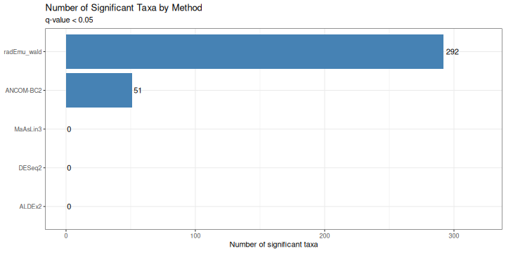

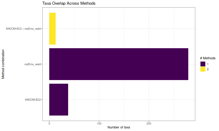
plot of chunk concordance_barplot

Overlap Between Methods (UpSet Plot)

# Create presence/absence matrix for significant taxa
sig_taxa_list <- results_spike |>
  filter(qvalue < 0.05) |>
  group_by(method) |>
  summarise(taxa = list(taxon)) |>
  tibble::deframe()

# Convert to binary matrix
all_taxa <- unique(unlist(sig_taxa_list))
sig_matrix <- sapply(sig_taxa_list, function(x) all_taxa %in% x)
rownames(sig_matrix) <- all_taxa

if (nrow(sig_matrix) > 0) {
  # UpSet-style visualization
  overlap_df <- as.data.frame(sig_matrix) |>
    rownames_to_column("taxon") |>
    pivot_longer(-taxon, names_to = "method", values_to = "significant") |>
    filter(significant) |>
    group_by(taxon) |>
    summarise(
      n_methods = n(),
      methods = paste(sort(method), collapse = " + ")
    )

  ggplot(overlap_df, aes(x = reorder(methods, n_methods), fill = factor(n_methods))) +
    geom_bar() +
    coord_flip() +
    scale_fill_viridis_d(name = "# Methods") +
    labs(
      title = "Taxa Overlap Across Methods",
      x = "Method combination",
      y = "Number of taxa"
    ) +
    theme_bw() +
    theme(legend.position = "right")
}

plot of chunk upset_plot

Pairwise Method Agreement

# Calculate Jaccard similarity between methods
methods <- unique(results_spike$method)
jaccard_matrix <- matrix(NA, length(methods), length(methods),
                        dimnames = list(methods, methods))

for (i in seq_along(methods)) {
  for (j in seq_along(methods)) {
    taxa_i <- results_spike$taxon[results_spike$method == methods[i] &
                                   results_spike$qvalue < 0.05]
    taxa_j <- results_spike$taxon[results_spike$method == methods[j] &
                                   results_spike$qvalue < 0.05]

    intersection <- length(intersect(taxa_i, taxa_j))
    union <- length(union(taxa_i, taxa_j))

    jaccard_matrix[i, j] <- if (union > 0) intersection / union else 0
  }
}

# Plot heatmap
jaccard_df <- as.data.frame(as.table(jaccard_matrix))
names(jaccard_df) <- c("Method1", "Method2", "Jaccard")

ggplot(jaccard_df, aes(x = Method1, y = Method2, fill = Jaccard)) +
  geom_tile() +
  geom_text(aes(label = round(Jaccard, 2)), color = "white", size = 4) +
  scale_fill_viridis_c(limits = c(0, 1)) +
  labs(
    title = "Pairwise Method Agreement (Jaccard Similarity)",
    subtitle = "Based on significant taxa (q < 0.05)",
    x = NULL, y = NULL
  ) +
  theme_bw() +
  theme(axis.text.x = element_text(angle = 45, hjust = 1))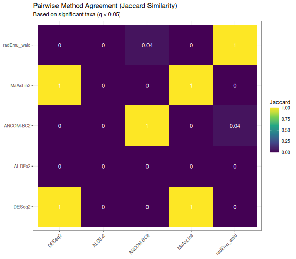

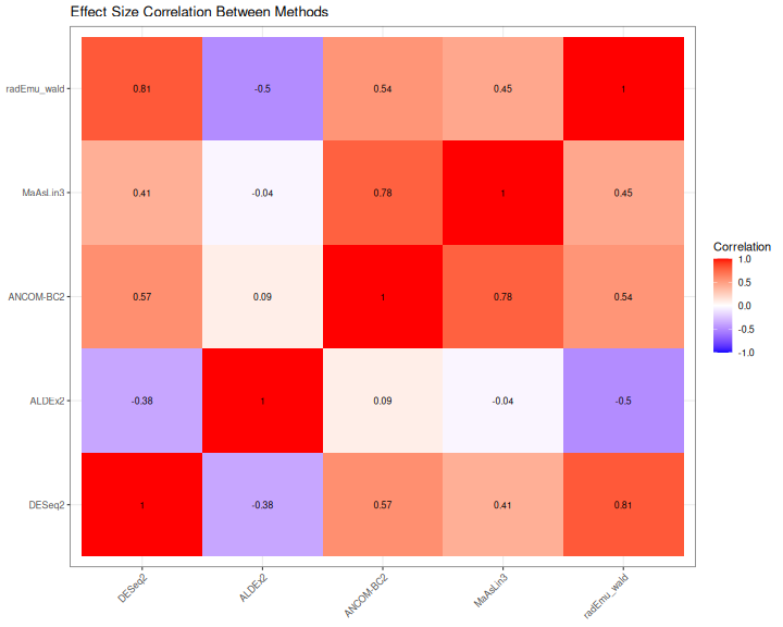
plot of chunk pairwise_agreement

Effect Size Comparison

Effect Size Correlation

# Wide format for effect sizes
effects_wide <- results_spike |>
  dplyr::select(taxon, method, effect) |>
  pivot_wider(names_from = method, values_from = effect)

# Pairwise scatter plots
if (ncol(effects_wide) > 2) {
  # Calculate correlations
  cor_matrix <- cor(effects_wide[, -1], use = "pairwise.complete.obs")

  # Plot correlation matrix
  cor_df <- as.data.frame(as.table(cor_matrix))
  names(cor_df) <- c("Method1", "Method2", "Correlation")

  p_cor <- ggplot(cor_df, aes(x = Method1, y = Method2, fill = Correlation)) +
    geom_tile() +
    geom_text(aes(label = round(Correlation, 2)), color = "black", size = 3) +
    scale_fill_gradient2(low = "blue", mid = "white", high = "red",
                        midpoint = 0, limits = c(-1, 1)) +
    labs(
      title = "Effect Size Correlation Between Methods",
      x = NULL, y = NULL
    ) +
    theme_bw() +
    theme(axis.text.x = element_text(angle = 45, hjust = 1))

  print(p_cor)
}

plot of chunk effect_correlation

Effect Size Distribution

ggplot(results_spike, aes(x = effect, fill = method)) +
  geom_density(alpha = 0.5) +
  facet_wrap(~method, scales = "free_y") +
  geom_vline(xintercept = 0, linetype = "dashed") +
  labs(
    title = "Distribution of Effect Sizes by Method",
    x = "Effect Size (log2 fold change)",
    y = "Density"
  ) +
  theme_bw() +
  theme(legend.position = "none")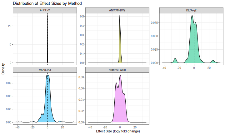

plot of chunk effect_distribution

FDR Control Assessment

Using our spike-in data, we can evaluate how well each method controls FDR.

# Get the actual spiked taxa (those with multiplied counts)
# We need to identify them from the multiply_counts_pq function
# For this, we'll use the taxa that were selected (stored during creation)

# Mark true positives
results_spike <- results_spike |>
  mutate(
    true_da = taxon %in% spike_taxa,
    called_da = qvalue < 0.05
  )

# Calculate performance metrics
performance <- results_spike |>
  group_by(method) |>
  summarise(
    TP = sum(true_da & called_da, na.rm = TRUE),
    FP = sum(!true_da & called_da, na.rm = TRUE),
    TN = sum(!true_da & !called_da, na.rm = TRUE),
    FN = sum(true_da & !called_da, na.rm = TRUE),
    .groups = "drop"
  ) |>
  mutate(
    Sensitivity = TP / (TP + FN),
    Specificity = TN / (TN + FP),
    FDR = FP / (TP + FP),
    Precision = TP / (TP + FP),
    F1 = 2 * (Precision * Sensitivity) / (Precision + Sensitivity)
  )

knitr::kable(
  performance |> 
    dplyr::select(method, TP, FP, FN, Sensitivity, FDR, F1),
  caption = "Performance metrics based on spike-in ground truth",
  digits = 3
)

Performance metrics based on spike-in ground truth
method	TP	FP	FN	Sensitivity	FDR	F1
ALDEx2	0	0	32	0.000	NaN	NaN
ANCOM-BC2	9	42	13	0.409	0.824	0.247
DESeq2	0	0	3	0.000	NaN	NaN
MaAsLin3	0	0	32	0.000	NaN	NaN
radEmu_wald	23	269	9	0.719	0.921	0.142

performance_long <- performance |>
  dplyr::select(method, Sensitivity, Specificity, FDR, F1) |>
  pivot_longer(-method, names_to = "Metric", values_to = "Value")

ggplot(performance_long, aes(x = method, y = Value, fill = Metric)) +
  geom_col(position = "dodge") +
  geom_hline(data = data.frame(Metric = "FDR", y = 0.05),
             aes(yintercept = y), linetype = "dashed", color = "red") +
  facet_wrap(~Metric, scales = "free_y") +
  labs(
    title = "Performance Metrics by Method",
    subtitle = "Red dashed line = nominal FDR (0.05)",
    x = NULL, y = "Value"
  ) +
  theme_bw() +
  theme(axis.text.x = element_text(angle = 45, hjust = 1),
        legend.position = "none")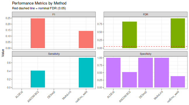

plot of chunk performance_plot

Volcano Plots Comparison

results_spike <- results_spike |>
  mutate(
    neg_log10_q = -log10(qvalue),
    significant = qvalue < 0.05,
    category = case_when(
      true_da & significant ~ "True Positive",
      !true_da & significant ~ "False Positive",
      true_da & !significant ~ "False Negative",
      TRUE ~ "True Negative"
    )
  )

ggplot(results_spike, aes(x = effect, y = neg_log10_q, color = category)) +
  geom_point(alpha = 0.6, size = 1.5) +
  geom_hline(yintercept = -log10(0.05), linetype = "dashed", color = "grey40") +
  geom_vline(xintercept = 0, color = "grey40") +
  scale_color_manual(values = c(
    "True Positive" = "forestgreen",
    "False Positive" = "red",
    "False Negative" = "orange",
    "True Negative" = "grey70"
  )) +
  facet_wrap(~method, scales = "free") +
  labs(
    title = "Volcano Plots by Method",
    subtitle = "Colors based on spike-in ground truth",
    x = "Effect Size",
    y = "-log10(q-value)",
    color = "Classification"
  ) +
  theme_bw() +
  theme(legend.position = "bottom")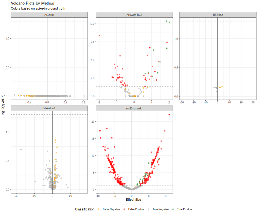

plot of chunk volcano_comparison

Real Data: HMP2 Antibiotics

Now we apply the methods to real data without known ground truth.

# Load HMP2 data
taxa_table_name <- system.file("extdata", "HMP2_taxonomy.tsv", package = "maaslin3")
taxa_table <- read.csv(taxa_table_name, sep = "\t", row.names = 1)

metadata_name <- system.file("extdata", "HMP2_metadata.tsv", package = "maaslin3")
metadata <- read.csv(metadata_name, sep = "\t", row.names = 1)

metadata$antibiotics <- factor(metadata$antibiotics, levels = c("No", "Yes"))

# Create phyloseq
otu <- otu_table(as.matrix(taxa_table), taxa_are_rows = FALSE)
sam <- sample_data(metadata)
species_names <- colnames(taxa_table)
tax_df <- data.frame(
  Species = species_names,
  Genus = sapply(strsplit(species_names, "_"), \(x) x[1]),
  row.names = species_names
)
tax <- tax_table(as.matrix(tax_df))
physeq_hmp2 <- phyloseq(otu, sam, tax)

# Convert to integer counts for count-based methods
# HMP2 data appears to be relative abundances, multiply by 1e6
otu_table(physeq_hmp2) <- otu_table(
  round(as.matrix(otu_table(physeq_hmp2)) * 1e6),
  taxa_are_rows = FALSE
)

cat("HMP2 Dataset:\n")
#> HMP2 Dataset:
cat("- Taxa:", ntaxa(physeq_hmp2), "\n")
#> - Taxa: 151
cat("- Samples:", nsamples(physeq_hmp2), "\n")
#> - Samples: 1527

results_hmp2 <- run_all_methods(
  physeq_hmp2,
  methods = c("ALDEx2", "ANCOM-BC2", "MaAsLin3", "radEmu"),
  group_var = "antibiotics",
  contrast_levels = c("Yes", "No"),
  verbose=TRUE,
  nclusters = 4
)

# Concordance plot
sig_hmp2 <- results_hmp2 |>
  filter(qvalue < 0.05) |>
  group_by(method) |>
  summarise(taxa = list(taxon)) |>
  tibble::deframe()

# Calculate consensus
consensus_hmp2 <- results_hmp2 |>
  filter(qvalue < 0.05) |>
  group_by(taxon) |>
  summarise(
    n_methods = n_distinct(method),
    methods = paste(sort(unique(method)), collapse = ", "),
    mean_effect = mean(effect, na.rm = TRUE)
  ) |>
  arrange(desc(n_methods), desc(abs(mean_effect)))

cat("\nTop consensus taxa (found by 4+ methods):\n")
#> 
#> Top consensus taxa (found by 4+ methods):
consensus_hmp2 |>
  filter(n_methods >= 2) |>
  head(15) |>
  knitr::kable(digits = 2)

taxon	n_methods	methods	mean_effect
Bacteroides_finegoldii	4	ALDEx2, ANCOM-BC2, MaAsLin3, radEmu_wald	1.27
Roseburia_intestinalis	4	ALDEx2, ANCOM-BC2, MaAsLin3, radEmu_wald	-1.14
GGB1680_SGB2312	3	ALDEx2, MaAsLin3, radEmu_wald	-9.09
Alistipes_dispar	3	ALDEx2, MaAsLin3, radEmu_wald	3.78
GGB3478_SGB14857	3	ALDEx2, MaAsLin3, radEmu_wald	3.19
Bifidobacterium_adolescentis	3	ANCOM-BC2, MaAsLin3, radEmu_wald	-2.24
Escherichia_coli	3	ANCOM-BC2, MaAsLin3, radEmu_wald	1.93
Klebsiella_pneumoniae	3	ALDEx2, MaAsLin3, radEmu_wald	1.78
Lachnospira_pectinoschiza	3	ANCOM-BC2, MaAsLin3, radEmu_wald	-1.26
Bacteroides_intestinalis	3	ALDEx2, ANCOM-BC2, radEmu_wald	0.92
Faecalibacterium_SGB15315	3	ALDEx2, ANCOM-BC2, radEmu_wald	-0.90
Roseburia_faecis	3	ALDEx2, ANCOM-BC2, radEmu_wald	-0.73
GGB3746_SGB5089	3	ALDEx2, ANCOM-BC2, radEmu_wald	-0.67
Clostridium_sp_AF36_4	3	ALDEx2, ANCOM-BC2, radEmu_wald	-0.56
Alistipes_SGB2313	2	MaAsLin3, radEmu_wald	-5.65

results_hmp2 |>
  mutate(significant = qvalue < 0.05) |>
  ggplot(aes(x = effect, y = -log10(qvalue), color = significant)) +
  geom_point(alpha = 0.5) +
  geom_hline(yintercept = -log10(0.05), linetype = "dashed") +
  scale_color_manual(values = c("FALSE" = "grey60", "TRUE" = "firebrick")) +
  facet_wrap(~method, scales = "free") +
  labs(
    title = "HMP2: Antibiotics Effect",
    x = "Effect Size",
    y = "-log10(q-value)"
  ) +
  theme_bw() +
  theme(legend.position = "bottom")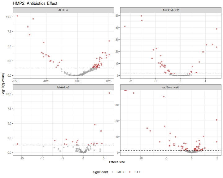

plot of chunk hmp2_volcano

Session Info

sessionInfo()
#> R version 4.6.0 (2026-04-24)
#> Platform: x86_64-pc-linux-gnu
#> Running under: Pop!_OS 24.04 LTS
#> 
#> Matrix products: default
#> BLAS:   /usr/lib/x86_64-linux-gnu/openblas-pthread/libblas.so.3 
#> LAPACK: /usr/lib/x86_64-linux-gnu/openblas-pthread/libopenblasp-r0.3.26.so;  LAPACK version 3.12.0
#> 
#> locale:
#>  [1] LC_CTYPE=en_US.UTF-8       LC_NUMERIC=C              
#>  [3] LC_TIME=en_US.UTF-8        LC_COLLATE=en_US.UTF-8    
#>  [5] LC_MONETARY=en_US.UTF-8    LC_MESSAGES=en_US.UTF-8   
#>  [7] LC_PAPER=en_US.UTF-8       LC_NAME=C                 
#>  [9] LC_ADDRESS=C               LC_TELEPHONE=C            
#> [11] LC_MEASUREMENT=en_US.UTF-8 LC_IDENTIFICATION=C       
#> 
#> time zone: Europe/Paris
#> tzcode source: system (glibc)
#> 
#> attached base packages:
#> [1] stats4    stats     graphics  grDevices utils     datasets  methods  
#> [8] base     
#> 
#> other attached packages:
#>  [1] BiocParallel_1.46.0         radEmu_2.3.2.0             
#>  [3] rlang_1.2.0                 magrittr_2.0.5             
#>  [5] Matrix_1.7-5                edgeR_4.10.1               
#>  [7] limma_3.68.4                DESeq2_1.52.0              
#>  [9] SummarizedExperiment_1.42.0 Biobase_2.72.0             
#> [11] MatrixGenerics_1.24.0       matrixStats_1.5.0          
#> [13] GenomicRanges_1.64.0        Seqinfo_1.2.0              
#> [15] IRanges_2.46.0              S4Vectors_0.50.1           
#> [17] BiocGenerics_0.58.1         generics_0.1.4             
#> [19] tibble_3.3.1                tidyr_1.3.2                
#> [21] ALDEx2_1.44.0               latticeExtra_0.6-31        
#> [23] lattice_0.22-9              zCompositions_1.6.1        
#> [25] survival_3.8-6              truncnorm_1.0-9            
#> [27] MASS_7.3-65                 doRNG_1.8.6.3              
#> [29] rngtools_1.5.2              foreach_1.5.2              
#> [31] patchwork_1.3.2             comparpq_0.1.3             
#> [33] S7_0.2.2                    MiscMetabar_0.16.8         
#> [35] dplyr_1.2.1                 ggplot2_4.0.3              
#> [37] phyloseq_1.56.0             knitr_1.51                 
#> 
#> loaded via a namespace (and not attached):
#>   [1] gld_2.6.8                       nnet_7.3-20                    
#>   [3] Biostrings_2.80.1               TH.data_1.1-5                  
#>   [5] vctrs_0.7.3                     maaslin3_1.4.0                 
#>   [7] energy_1.7-12                   digest_0.6.39                  
#>   [9] png_0.1-9                       shape_1.4.6.1                  
#>  [11] proxy_0.4-29                    Exact_3.3                      
#>  [13] ggrepel_0.9.8                   deldir_2.0-4                   
#>  [15] permute_0.9-10                  fontLiberation_0.1.0           
#>  [17] reshape2_1.4.5                  withr_3.0.2                    
#>  [19] psych_2.6.5                     ecodive_2.2.6                  
#>  [21] xfun_0.58                       ggfun_0.2.0                    
#>  [23] memoise_2.0.1                   ggbeeswarm_0.7.3               
#>  [25] emmeans_2.0.3                   systemfonts_1.3.2              
#>  [27] ragg_1.5.2                      tidytree_0.4.7                 
#>  [29] zoo_1.8-15                      GlobalOptions_0.1.4            
#>  [31] gtools_3.9.5                    logging_0.10-111               
#>  [33] Formula_1.2-5                   otel_0.2.0                     
#>  [35] httr_1.4.8                      nanonext_1.9.1                 
#>  [37] kmer_1.1.3                      rstudioapi_0.19.0              
#>  [39] ggalluvial_0.12.6               base64enc_0.1-6                
#>  [41] curl_7.1.0                      ScaledMatrix_1.20.0            
#>  [43] quadprog_1.5-8                  SparseArray_1.12.2             
#>  [45] pracma_2.4.6                    xtable_1.8-8                   
#>  [47] stringr_1.6.0                   ade4_1.7-24                    
#>  [49] doParallel_1.0.17               evaluate_1.0.5                 
#>  [51] S4Arrays_1.12.0                 Rfast_2.1.5.2                  
#>  [53] BiocFileCache_3.2.0             hms_1.1.4                      
#>  [55] irlba_2.3.7                     colorspace_2.1-2               
#>  [57] filelock_1.0.3                  readxl_1.5.0                   
#>  [59] readr_2.2.0                     viridis_0.6.5                  
#>  [61] ggtree_4.2.0                    DECIPHER_3.8.0                 
#>  [63] scuttle_1.22.0                  class_7.3-23                   
#>  [65] Hmisc_5.2-5                     pillar_1.11.1                  
#>  [67] nlme_3.1-169                    iterators_1.0.14               
#>  [69] decontam_1.32.0                 compiler_4.6.0                 
#>  [71] beachmat_2.28.0                 stringi_1.8.7                  
#>  [73] biomformat_1.40.0               DescTools_0.99.60              
#>  [75] minqa_1.2.8                     plyr_1.8.9                     
#>  [77] crayon_1.5.3                    abind_1.4-8                    
#>  [79] scater_1.40.1                   gridGraphics_0.5-1             
#>  [81] locfit_1.5-9.12                 haven_2.5.5                    
#>  [83] bit_4.6.0                       mia_1.20.0                     
#>  [85] rootSolve_1.8.2.4               sandwich_3.1-1                 
#>  [87] divent_0.5-4                    codetools_0.2-20               
#>  [89] multcomp_1.4-30                 textshaping_1.0.5              
#>  [91] directlabels_2026.4.23          BiocSingular_1.28.0            
#>  [93] e1071_1.7-17                    lmom_3.3                       
#>  [95] multtest_2.68.0                 MultiAssayExperiment_1.38.0    
#>  [97] splines_4.6.0                   circlize_0.4.18                
#>  [99] Rcpp_1.1.1-1.1                  dbplyr_2.5.2                   
#> [101] sparseMatrixStats_1.24.0        cellranger_1.1.0               
#> [103] interp_1.1-6                    blob_1.3.0                     
#> [105] utf8_1.2.6                      lme4_2.0-1                     
#> [107] fs_2.1.0                        checkmate_2.3.4                
#> [109] DelayedMatrixStats_1.34.0       Rdpack_2.6.6                   
#> [111] expm_1.0-0                      gsl_2.1-9                      
#> [113] ggplotify_0.1.3                 estimability_1.5.1             
#> [115] scam_1.2-22                     statmod_1.5.2                  
#> [117] tzdb_0.5.0                      pkgconfig_2.0.3                
#> [119] tools_4.6.0                     cachem_1.1.0                   
#> [121] rbibutils_2.4.1                 RSQLite_3.53.1                 
#> [123] viridisLite_0.4.3               DBI_1.3.0                      
#> [125] numDeriv_2016.8-1.1             phylogram_2.1.0                
#> [127] zigg_0.0.2                      fastmap_1.2.0                  
#> [129] rmarkdown_2.31                  scales_1.4.0                   
#> [131] grid_4.6.0                      coda_0.19-4.1                  
#> [133] rpart_4.1.27                    farver_2.1.2                   
#> [135] reformulas_0.4.4                mgcv_1.9-4                     
#> [137] foreign_0.8-91                  cli_3.6.6                      
#> [139] purrr_1.2.2                     lifecycle_1.0.5                
#> [141] mvtnorm_1.4-1                   bluster_1.22.0                 
#> [143] backports_1.5.1                 mirai_2.7.1                    
#> [145] gtable_0.3.6                    ANCOMBC_2.14.0                 
#> [147] parallel_4.6.0                  ape_5.8-1                      
#> [149] jsonlite_2.0.0                  multcompView_0.1-11            
#> [151] bit64_4.8.2                     Rtsne_0.17                     
#> [153] yulab.utils_0.2.4               vegan_2.7-5                    
#> [155] MIDASim_2.0                     BiocNeighbors_2.6.0            
#> [157] TreeSummarizedExperiment_2.20.0 RcppParallel_5.1.11-2          
#> [159] formattable_0.2.1               lazyeval_0.2.3                 
#> [161] htmltools_0.5.9                 collapse_2.1.7                 
#> [163] rappdirs_0.3.4                  glue_1.8.1                     
#> [165] optparse_1.8.2                  httr2_1.2.2                    
#> [167] XVector_0.52.0                  gdtools_0.5.1                  
#> [169] treeio_1.36.1                   mnormt_2.1.2                   
#> [171] jpeg_0.1-11                     gridExtra_2.3                  
#> [173] boot_1.3-32                     igraph_2.3.2                   
#> [175] R6_2.6.1                        MicrobiomeBenchmarkData_1.14.0 
#> [177] SingleCellExperiment_1.34.0     ggiraph_0.9.6                  
#> [179] forcats_1.0.1                   labeling_0.4.3                 
#> [181] cluster_2.1.8.2                 aplot_0.2.9                    
#> [183] nloptr_2.2.1                    DirichletMultinomial_1.54.0    
#> [185] DelayedArray_0.38.2             tidyselect_1.2.1               
#> [187] vipor_0.4.7                     htmlTable_2.5.0                
#> [189] microbiome_1.34.0               fontBitstreamVera_0.1.1        
#> [191] rsvd_1.0.5                      fontquiver_0.2.1               
#> [193] data.table_1.18.4               htmlwidgets_1.6.4              
#> [195] RColorBrewer_1.1-3              lmerTest_3.2-1                 
#> [197] ggnewscale_0.5.2                beeswarm_0.4.0

Adrien Taudière

2026-06-18

Introduction

Setup

Helper Functions

Dataset: Simulated Spike-in Data

Approach A: `multiply_counts_pq` with compensation

Approach B: `permute_da_pq` (strict library size preservation)

Approach C: `midasim_pq` (realistic simulation)

Use Approach A for benchmark

Run All Methods

Concordance Analysis

Number of Significant Taxa

Overlap Between Methods (UpSet Plot)

Pairwise Method Agreement

Effect Size Comparison

Effect Size Correlation

Effect Size Distribution

FDR Control Assessment

Volcano Plots Comparison

Real Data: HMP2 Antibiotics

Session Info

Benchmarking Differential Abundance Methods

Adrien Taudière

2026-06-18

Introduction

Setup

Helper Functions

Dataset: Simulated Spike-in Data

Approach A: multiply_counts_pq with compensation

Approach B: permute_da_pq (strict library size preservation)

Approach C: midasim_pq (realistic simulation)

Use Approach A for benchmark

Run All Methods

Concordance Analysis

Number of Significant Taxa

Overlap Between Methods (UpSet Plot)

Pairwise Method Agreement

Effect Size Comparison

Effect Size Correlation

Effect Size Distribution

FDR Control Assessment

Volcano Plots Comparison

Real Data: HMP2 Antibiotics

Session Info

Approach A: `multiply_counts_pq` with compensation

Approach B: `permute_da_pq` (strict library size preservation)

Approach C: `midasim_pq` (realistic simulation)