Getting Started with greenAlgoR

Introduction

The greenAlgoR package provides tools to estimate the carbon footprint and energy consumption of computational tasks in R. This package is based on the Green Algorithms framework (Lannelongue, Grealey, and Inouye 2021), which provides a standardized approach to quantifying the environmental impact of computational research.

Understanding the carbon footprint of our computational work is increasingly important as we strive to make research more sustainable. The greenAlgoR package makes it easy to:

Calculate CO2 emissions from R computations
Compare different computational approaches
Optimize code for environmental impact
Track carbon footprint across research projects

Installation

# Install from GitHub (development version)
if (!require("devtools", quietly = TRUE)) {
  install.packages("devtools")
}
devtools::install_github("adrientaudiere/greenAlgoR")

library(greenAlgoR)
library(ggplot2)

Basic Usage

Calculating Carbon Footprint

The main function ga_footprint() calculates the carbon footprint based on several parameters:

# Calculate footprint for a 2-hour computation
result <- ga_footprint(
  runtime_h = 2,
  location_code = "WORLD", # Global average carbon intensity
  n_cores = 4,
  TDP_per_core = 15, # Thermal Design Power per core in Watts
  memory_ram = 16 # RAM in GB
)

# View key results
cat("Carbon footprint:", result$carbon_footprint_total_gCO2, "g CO2\n")
#> Carbon footprint: 104.6455 g CO2
cat("Energy needed:", result$energy_needed_kWh, "kWh\n")
#> Energy needed: 0.2203064 kWh

Understanding the Results

The function returns a comprehensive list with detailed breakdown:

# View all available information
names(result)
#>  [1] "runtime_h"                   "location_code"              
#>  [3] "TDP_per_core"                "n_cores"                    
#>  [5] "cpu_model"                   "memory_ram"                 
#>  [7] "power_draw_per_gb"           "usage core"                 
#>  [9] "carbon_intensity"            "PUE"                        
#> [11] "PSF"                         "power_draw_for_cores_kWh"   
#> [13] "power_draw_for_memory_kWh"   "energy_needed_kWh"          
#> [15] "carbon_footprint_cores"      "carbon_footprint_memory"    
#> [17] "carbon_footprint_total_gCO2" "ref_value"

# Key components of carbon footprint
cat("CPU contribution:", result$carbon_footprint_cores, "g CO2\n")
#> CPU contribution: 95.19 g CO2
cat("Memory contribution:", result$carbon_footprint_memory, "g CO2\n")
#> Memory contribution: 9.45554 g CO2
cat("Total footprint:", result$carbon_footprint_total_gCO2, "g CO2\n")
#> Total footprint: 104.6455 g CO2

Location-Specific Carbon Intensity

Carbon intensity varies significantly by location due to different energy sources:

# Compare carbon footprint across different locations
locations <- c("FR", "WORLD", "US", "CN", "NO")
footprints <- sapply(locations, function(loc) {
  ga_footprint(runtime_h = 1, location_code = loc, n_cores = 2)$carbon_footprint_total_gCO2
})

# Create comparison data frame
comparison_df <- data.frame(
  Location = locations,
  CO2_emissions = footprints
)

print(comparison_df)
#>       Location CO2_emissions
#> FR          FR     2.5903478
#> WORLD    WORLD    23.9940561
#> US          US    21.4148213
#> CN          CN    27.1461173
#> NO          NO     0.3849152

# Visualize the comparison
ggplot(comparison_df, aes(x = reorder(Location, CO2_emissions), y = CO2_emissions)) +
  geom_col(fill = "steelblue", alpha = 0.7) +
  labs(
    title = "Carbon Footprint by Location",
    subtitle = "1-hour computation with 2 cores",
    x = "Location",
    y = "CO2 Emissions (g)",
    caption = "Based on regional carbon intensity differences"
  ) +
  theme_minimal() +
  theme(axis.text.x = element_text(angle = 45, hjust = 1))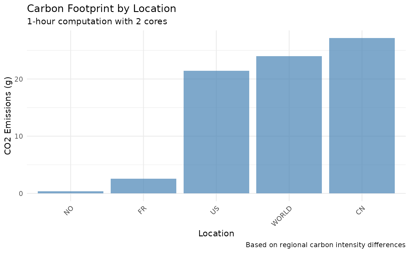

Bar plot comparing carbon footprint across different locations for a 1-hour computation with 2 cores.

Hardware Configuration

Different hardware configurations have varying environmental impacts:

# Compare different CPU configurations
cpu_configs <- data.frame(
  Config = c("Laptop", "Workstation", "Server"),
  Cores = c(4, 8, 16),
  TDP_per_core = c(10, 15, 25),
  Memory = c(8, 32, 64)
)

# Calculate footprint for each configuration
cpu_configs$Footprint <- mapply(function(cores, tdp, mem) {
  ga_footprint(
    runtime_h = 1,
    n_cores = cores,
    TDP_per_core = tdp,
    memory_ram = mem
  )$carbon_footprint_total_gCO2
}, cpu_configs$Cores, cpu_configs$TDP_per_core, cpu_configs$Memory)

print(cpu_configs)
#>        Config Cores TDP_per_core Memory Footprint
#> 1      Laptop     4           10      8  34.09389
#> 2 Workstation     8           15     32 104.64554
#> 3      Server    16           25     64 336.21108

Current R Session Footprint

You can easily calculate the carbon footprint of your current R session:

# Get current session footprint
session_fp <- ga_footprint(runtime_h = "session")

cat("Current session footprint:", session_fp$carbon_footprint_total_gCO2, "g CO2\n")
#> Current session footprint: 0.01303559 g CO2
cat("Session runtime:", session_fp$runtime_h, "hours\n")
#> Session runtime: 0.0009005556 hours

Visualization with Reference Values

The package includes reference values to put your footprint in context:

# Calculate footprint with reference values
result_with_ref <- ga_footprint(
  runtime_h = 2,
  n_cores = 4,
  memory_ram = 16,
  add_ref_values = TRUE
)

# Create visualization comparing to reference values
ref_data <- result_with_ref$ref_value
ref_data$is_computation <- FALSE
ref_data$is_computation[ref_data$variable == "Total"] <- TRUE

# Add our computation to the data
computation_data <- data.frame(
  variable = "Your Computation",
  value = result_with_ref$carbon_footprint_total_gCO2,
  prop_footprint = NA,
  is_computation = TRUE
)

plot_data <- rbind(
  ref_data[, c("variable", "value", "is_computation")],
  computation_data[, c("variable", "value", "is_computation")]
)
plot_data$value <- as.numeric(plot_data$value)

ggplot(plot_data, aes(
  x = reorder(variable, value), y = value,
  fill = is_computation
)) +
  geom_col(alpha = 0.8) +
  scale_fill_manual(
    values = c("FALSE" = "lightblue", "TRUE" = "darkred"),
    name = "Type",
    labels = c("Reference", "Your Computation")
  ) +
  scale_y_log10() +
  coord_flip() +
  labs(
    title = "Carbon Footprint Comparison",
    subtitle = "Your computation vs. reference activities",
    x = "Activity",
    y = "CO2 Emissions (g, log scale)",
    caption = "Reference values help contextualize computational impact"
  ) +
  theme_minimal() +
  theme(legend.position = "bottom")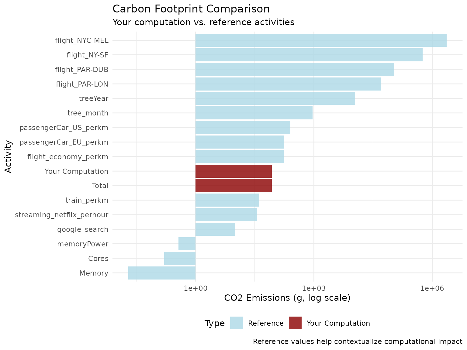

Footprint value compared to references values such as 1 hour of Netflix streaming and a fly from London to Paris.

Best Practices

Choose efficient algorithms: Optimize your code to reduce runtime
Consider location: Run computations in regions with cleaner energy
Right-size resources: Use appropriate CPU/memory for your task
Monitor regularly: Track footprint across projects
Share awareness: Include carbon footprint in research reporting

Next Steps

Explore the ga_targets() function for pipeline analysis
Check the package documentation for advanced configuration options
Consider the carbon impact in your research workflow decisions

References

Lannelongue, Loïc, Jason Grealey, and Michael Inouye. 2021. “Green Algorithms: Quantifying the Carbon Footprint of Computation.” Advanced Science 8 (12): 2100707. https://doi.org/10.1002/advs.202100707.

Adrien Taudière

2025-09-24