Using greenAlgoR with targets Pipelines

Introduction

The targets package (landau_targets_2021?) provides a powerful framework for reproducible computational workflows in R. The greenAlgoR package seamlessly integrates with targets to help you understand the environmental impact of your entire data analysis pipeline.

This vignette demonstrates how to:

Calculate carbon footprint for complete targets pipelines
Identify the most carbon-intensive steps in your workflow
Optimize pipelines for environmental efficiency

Setup

library(greenAlgoR)
library(targets)
library(ggplot2)

Basic targets Integration

The ga_targets() function analyzes your targets pipeline and calculates the total carbon footprint based on:

Runtime of each target
Memory usage patterns
Storage requirements (optional)

Simple Example

# Create a simple targets example
tar_dir({ # tar_dir() runs code from a temp dir for CRAN compatibility

  # Define a simple pipeline
  tar_script(
    {
      library(targets)

      list(
        tar_target(
          name = data_prep,
          command = {
            # Simulate data preparation (2 seconds)
            Sys.sleep(2)
            data.frame(x = rnorm(1000), y = rnorm(1000))
          }
        ),
        tar_target(
          name = analysis,
          command = {
            # Simulate analysis (1 second)
            Sys.sleep(1)
            lm(y ~ x, data = data_prep)
          }
        ),
        tar_target(
          name = visualization,
          command = {
            # Simulate plotting (0.5 seconds)
            Sys.sleep(0.5)
            plot(data_prep$x, data_prep$y)
            "plot_completed"
          }
        )
      )
    },
    ask = FALSE
  )

  # Run the pipeline
  tar_make()

  # Get metadata
  metadata <- tar_meta()
  print(metadata[, c("name", "seconds", "bytes")])

  # Calculate carbon footprint
  pipeline_footprint <- ga_targets(
    tar_meta_raw = metadata,
    location_code = "WORLD",
    n_cores = 2,
    TDP_per_core = 15,
    memory_ram = 8
  )

  cat(
    "Pipeline carbon footprint:",
    pipeline_footprint$carbon_footprint_total_gCO2, "g CO2\n"
  )
  cat("Total runtime:", pipeline_footprint$runtime_h * 3600, "seconds\n")
})
#> + data_prep dispatched
#> ✔ data_prep completed [2s, 15.52 kB]
#> + analysis dispatched
#> ✔ analysis completed [1s, 47.54 kB]
#> + visualization dispatched
#> ✔ visualization completed [533ms, 67 B]
#> ✔ ended pipeline [3.7s, 3 completed, 0 skipped]
#> # A tibble: 3 × 3
#>   name          seconds bytes
#>   <chr>           <dbl> <dbl>
#> 1 data_prep       2.00  15523
#> 2 analysis        1.00  47544
#> 3 visualization   0.533    67
#> Pipeline carbon footprint: 0.02572536 g CO2
#> Total runtime: 3.54 seconds

Advanced Pipeline Analysis

For more complex pipelines, you can get detailed insights:

tar_dir({
  # Create a more complex pipeline
  tar_script(
    {
      library(targets)

      simulate_computation <- function(duration, size = 1000) {
        Sys.sleep(duration)
        matrix(rnorm(size * size), nrow = size)
      }

      list(
        tar_target(small_task, simulate_computation(0.5, 100)),
        tar_target(medium_task, simulate_computation(2, 500)),
        tar_target(large_task, simulate_computation(5, 1000)),
        tar_target(
          combined_analysis,
          {
            # Combine results
            result <- list(
              small = summary(small_task),
              medium = summary(medium_task),
              large = summary(large_task)
            )
            Sys.sleep(1) # Additional processing time
            result
          }
        )
      )
    },
    ask = FALSE
  )

  tar_make()
  metadata <- tar_meta()

  # Calculate footprint with storage estimation
  detailed_footprint <- ga_targets(
    tar_meta_raw = metadata,
    location_code = "FR", # France has relatively low carbon intensity
    n_cores = 4,
    TDP_per_core = 20,
    memory_ram = 16,
    add_storage_estimation = TRUE
  )

  # Display breakdown
  cat("Total CO2 emissions:", detailed_footprint$carbon_footprint_total_gCO2, "g\n")
  cat("CPU contribution:", detailed_footprint$carbon_footprint_cores, "g\n")
  cat("Memory contribution:", detailed_footprint$carbon_footprint_memory, "g\n")

  if (!is.null(detailed_footprint$power_draw_storage_kWh)) {
    storage_co2 <- detailed_footprint$carbon_intensity * detailed_footprint$power_draw_storage_kWh
    cat("Storage contribution:", storage_co2, "g\n")
  }
})
#> + large_task dispatched
#> ✔ large_task completed [5s, 7.68 MB]
#> + medium_task dispatched
#> ✔ medium_task completed [2s, 1.92 MB]
#> + small_task dispatched
#> ✔ small_task completed [502ms, 76.87 kB]
#> + combined_analysis dispatched
#> ✔ combined_analysis completed [1.4s, 49.99 kB]
#> ✔ ended pipeline [9.5s, 4 completed, 0 skipped]
#> Total CO2 emissions: 0.0182604 g
#> CPU contribution: 0.0169924 g
#> Memory contribution: 0.001265934 g
#> Storage contribution: 2.065548e-06 g

Comparing Different Configurations

You can compare how different hardware configurations affect your pipeline’s carbon footprint:

tar_dir({
  # Use the same pipeline as above
  tar_script(
    {
      library(targets)

      simulate_computation <- function(duration, size = 1000) {
        Sys.sleep(duration)
        matrix(rnorm(size * size), nrow = size)
      }

      list(
        tar_target(task1, simulate_computation(1, 200)),
        tar_target(task2, simulate_computation(2, 300)),
        tar_target(task3, simulate_computation(1.5, 250))
      )
    },
    ask = FALSE
  )

  tar_make()
  metadata <- tar_meta()

  # Compare different configurations
  configs <- data.frame(
    Config = c("Laptop", "Desktop", "Server"),
    Cores = c(2, 8, 16),
    TDP = c(10, 15, 25),
    RAM = c(8, 16, 64),
    Location = c("WORLD", "FR", "NO") # Different locations
  )

  # Calculate footprint for each configuration
  configs$CO2_emissions <- mapply(function(cores, tdp, ram, loc) {
    ga_targets(
      tar_meta_raw = metadata,
      n_cores = cores,
      TDP_per_core = tdp,
      memory_ram = ram,
      location_code = loc
    )$carbon_footprint_total_gCO2
  }, configs$Cores, configs$TDP, configs$RAM, configs$Location)

  print(configs)
})
#> + task1 dispatched
#> ✔ task1 completed [1s, 307.24 kB]
#> + task2 dispatched
#> ✔ task2 completed [2s, 691.03 kB]
#> + task3 dispatched
#> ✔ task3 completed [1.5s, 480.03 kB]
#> ✔ ended pipeline [4.7s, 3 completed, 0 skipped]
#>    Config Cores TDP RAM Location CO2_emissions
#> 1  Laptop     2  10   8    WORLD    0.02286206
#> 2 Desktop     8  15  16       FR    0.01352859
#> 3  Server    16  25  64       NO    0.00676439

Visualizing Pipeline Carbon Footprint

Create comprehensive visualizations of your pipeline’s environmental impact:

tar_dir({
  # Create pipeline and get footprint with reference values
  tar_script(
    {
      library(targets)
      list(
        tar_target(data_load, {
          Sys.sleep(1)
          rnorm(5000)
        }),
        tar_target(preprocessing, {
          Sys.sleep(3)
          scale(data_load)
        }),
        tar_target(modeling, {
          Sys.sleep(5)
          lm(data_load ~ seq_along(data_load))
        }),
        tar_target(postprocessing, {
          Sys.sleep(2)
          summary(modeling)
        })
      )
    },
    ask = FALSE
  )

  tar_make()
  metadata <- tar_meta()

  pipeline_result <- ga_targets(
    tar_meta_raw = metadata,
    location_code = "WORLD",
    n_cores = 4,
    memory_ram = 16,
    add_ref_values = TRUE
  )

  # Create comprehensive visualization
  ref_data <- pipeline_result$ref_value
  ref_data$category <- "Reference Activities"

  # Add pipeline data
  pipeline_data <- data.frame(
    variable = "Your Pipeline",
    value = pipeline_result$carbon_footprint_total_gCO2,
    prop_footprint = NA,
    category = "Your Computation"
  )

  # Combine data
  plot_data <- rbind(
    ref_data[, c("variable", "value", "category")],
    pipeline_data[, c("variable", "value", "category")]
  )
  plot_data$value <- as.numeric(plot_data$value)

  # Create the plot
  ggplot(plot_data, aes(
    x = reorder(variable, value), y = value,
    fill = category
  )) +
    geom_col(alpha = 0.8) +
    scale_fill_manual(
      values = c(
        "Reference Activities" = "lightblue",
        "Your Computation" = "darkgreen"
      ),
      name = "Type"
    ) +
    scale_y_log10() +
    coord_flip() +
    labs(
      title = "Carbon Footprint of targets Pipeline",
      subtitle = paste(
        "Total emissions:",
        round(pipeline_result$carbon_footprint_total_gCO2, 2),
        "g CO2"
      ),
      x = "Activity",
      y = "CO2 Emissions (g, log scale)",
      caption = "Comparison with everyday reference activities"
    ) +
    theme_minimal() +
    theme(
      legend.position = "bottom",
      plot.title = element_text(size = 14, face = "bold"),
      plot.subtitle = element_text(size = 12)
    )
})
#> + data_load dispatched
#> ✔ data_load completed [1s, 38.47 kB]
#> + modeling dispatched
#> ✔ modeling completed [5s, 238.68 kB]
#> + preprocessing dispatched
#> ✔ preprocessing completed [3s, 38.59 kB]
#> + postprocessing dispatched
#> ✔ postprocessing completed [2s, 77.94 kB]
#> ✔ ended pipeline [11.2s, 4 completed, 0 skipped]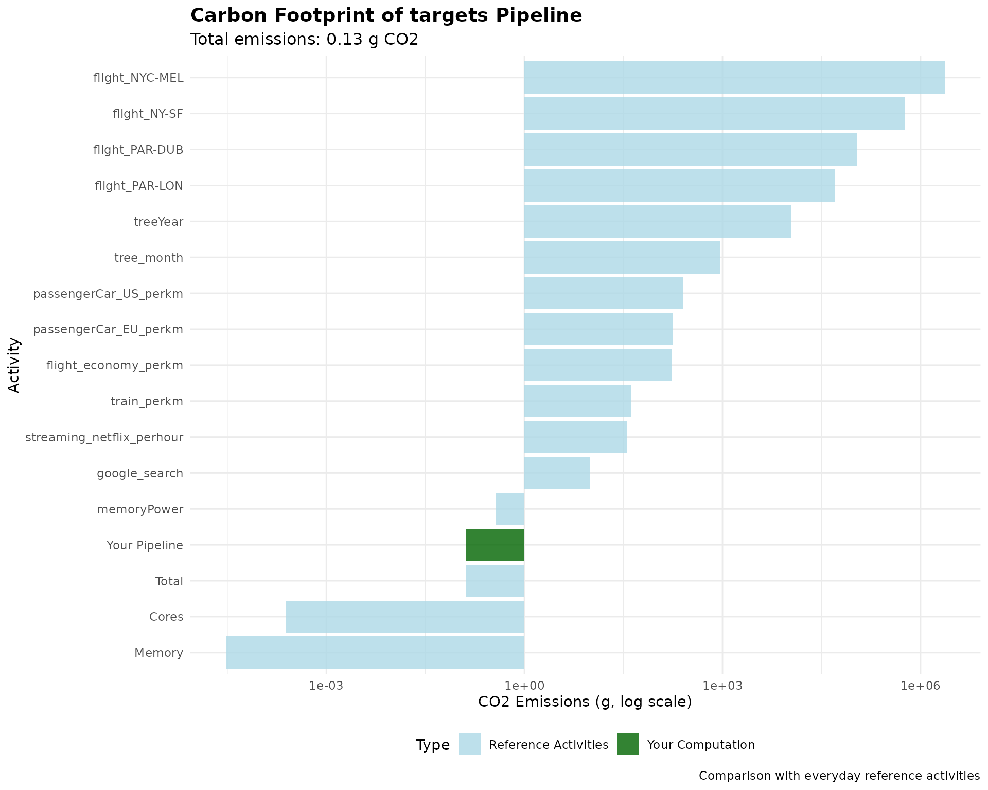

Footprint value compared to references values such as 1 hour of Netflix streaming and a fly from London to Paris.

Target-Level Analysis

For detailed optimization, you might want to analyze individual targets:

tar_dir({
  tar_script(
    {
      library(targets)
      list(
        tar_target(quick_task, {
          Sys.sleep(0.5)
          "done"
        }),
        tar_target(slow_task, {
          Sys.sleep(10)
          "done"
        }),
        tar_target(memory_intensive, {
          # Simulate memory-intensive task
          big_matrix <- matrix(rnorm(1000 * 1000), nrow = 1000)
          Sys.sleep(3)
          summary(big_matrix)
        })
      )
    },
    ask = FALSE
  )

  tar_make()
  metadata <- tar_meta()

  # Analyze each target separately
  target_analysis <- data.frame(
    Target = metadata$name,
    Runtime_sec = metadata$seconds,
    Memory_MB = metadata$bytes / (1024^2),
    stringsAsFactors = FALSE
  )

  # Calculate individual footprints (simplified)
  target_analysis$CO2_estimate <- sapply(metadata$seconds, function(sec) {
    ga_footprint(
      runtime_h = sec / 3600,
      n_cores = 2,
      memory_ram = 8
    )$carbon_footprint_total_gCO2
  })

  print(target_analysis)

  # Identify the most carbon-intensive target
  most_intensive <- target_analysis[which.max(target_analysis$CO2_estimate), ]
  cat(
    "\nMost carbon-intensive target:", most_intensive$Target,
    "(", round(most_intensive$CO2_estimate, 3), "g CO2 )\n"
  )
})
#> + memory_intensive dispatched
#> ✔ memory_intensive completed [3.3s, 31.13 kB]
#> + quick_task dispatched
#> ✔ quick_task completed [501ms, 57 B]
#> + slow_task dispatched
#> ✔ slow_task completed [10s, 57 B]
#> ✔ ended pipeline [13.9s, 3 completed, 0 skipped]
#>             Target Runtime_sec    Memory_MB CO2_estimate
#> 1 memory_intensive       3.281 2.968979e-02  0.019505440
#> 2       quick_task       0.501 5.435944e-05  0.002978429
#> 3        slow_task      10.011 5.435944e-05  0.059515075
#> 
#> Most carbon-intensive target: slow_task ( 0.06 g CO2 )

Best Practices for Sustainable Pipelines

Profile your pipeline: Use tar_meta() to identify bottlenecks
Optimize slow targets: Focus on reducing runtime of carbon-intensive steps
Cache efficiently: Use targets caching to avoid re-running expensive computations
Choose appropriate hardware: Match computational resources to task requirements
Consider location: Run pipelines in regions with cleaner energy if possible

Integration with Workflow

Include carbon footprint reporting as part of your standard pipeline:

# Add to your _targets.R file
tar_target(
  pipeline_footprint,
  {
    # Calculate footprint after pipeline completion
    footprint <- ga_targets(location_code = "FR")

    # Log the results
    cat(
      "Pipeline carbon footprint:",
      footprint$carbon_footprint_total_gCO2, "g CO2\n"
    )

    # Save for reporting
    saveRDS(footprint, "results/carbon_footprint.rds")

    footprint
  }
)

Conclusion

Integrating greenAlgoR with targets provides a powerful way to understand and optimize the environmental impact of your computational workflows. By regularly monitoring carbon footprint, you can make informed decisions about computational efficiency and contribute to more sustainable research practices.

Adrien Taudière

2025-09-24