Overview
Riley et al. 2025 (https://doi.org/10.1186/s12915-025-02284-x) propose the concept of species bound cluster (SBC) which are defined as “clusters that include all and only ESVs assigned to one species, the sequence similarity threshold can vary between these clusters”.
d_f_ab <- subset_taxa_pq(data_fungi, taxa_sums(data_fungi) > 50)Compute intra-taxonomic names distance
intra_taxn_dist <- intra_taxnames_dist(d_f_ab, verbose = FALSE)

intra_taxn_dist |>
  filter(n_taxa > 1) |>
  arrange(desc(n_taxa)) |>
  select(-taxnames) |>
  head(10)
#> n_taxa mean_dist min_dist max_dist
#> Hyperphyscia adglutinata 15 0.1853030 0.003300330 0.3940397
#> Dacrymyces stenosporus 14 0.2673166 0.003278689 0.4824281
#> Eutypa spinosa 13 0.1797748 0.006389776 0.3079470
#> Stereum ostrea 13 0.1636422 0.005602241 0.4068966
#> Scytalidium lignicola 13 0.2563321 0.003205128 0.4700315
#> Penicillium brevicompactum 13 0.2586561 0.003257329 0.4899329
#> Scheffersomyces lignosus 11 0.2536107 0.005882353 0.4980843
#> Angustimassarina acerina 10 0.2943042 0.003389831 0.4691358
#> Xylodon raduloides 9 0.2416071 0.003030303 0.3971631
#> Pertusaria leioplaca 9 0.3217032 0.005602241 0.4166667Cluster taxa into SBC
sbc_clusters <- cluster_sbc(d_f_ab, verbose = FALSE)

track_wkflow(list(
  "Raw physeq" = data_fungi,
  "Abundant taxa" = subset_taxa_pq(data_fungi, taxa_sums(data_fungi) > 500),
  "SBC" = sbc_clusters$physeq_SBC
)) |>
  knitr::kable()
<!-- KNITR_ASIS_OUTPUT_TOKEN -->
| | nb_sequences| nb_clusters| nb_samples|
|:-------------|------------:|-----------:|----------:|
|Raw physeq | 1839124| 1420| 185|
|Abundant taxa | 1660524| 420| 185|
|SBC | 345218| 135| 178|
<!-- KNITR_ASIS_OUTPUT_TOKEN -->```
``` r
sbc_clusters$summary#> n_taxnames n_taxa n_unassigned n_already_SBC n_taxa_to_cluster
#> 1 252 1334 720 147 467
#> avg_cluster_size avg_cluster_size_excluding_singleton n_new_SBC n_SBC mean_d
#> 1 2.177305 3.459259 135 282 3.2
#> median_d
#> 1 3
summary_plot_pq(sbc_clusters$physeq_SBC)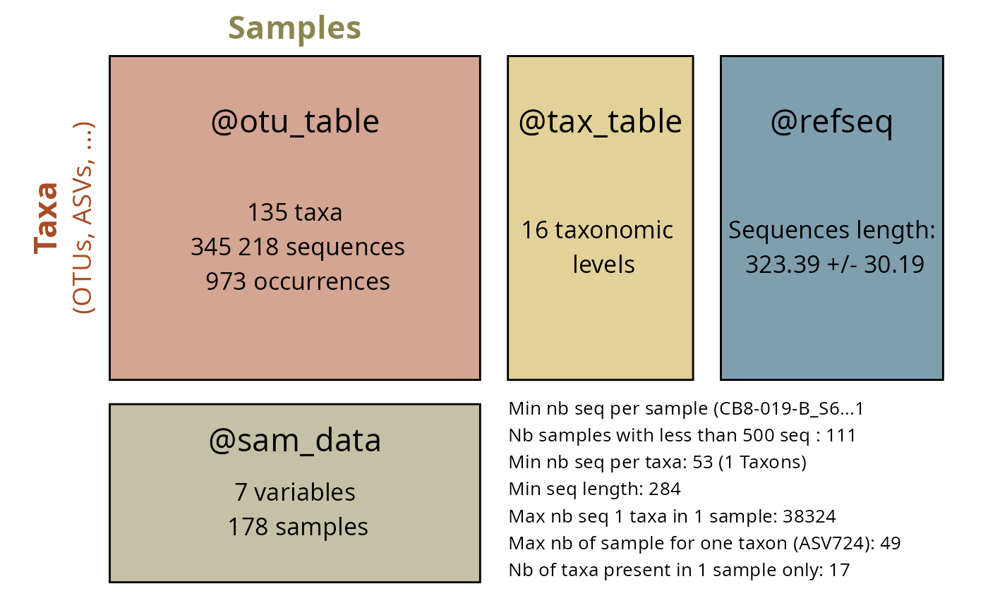
Visualize results
left_join(intra_taxn_dist, sbc_clusters$d_per_taxnames, by = "taxnames") |>
  filter(!is.na(optimal_d)) |>
  ggplot(aes(x = optimal_d, y = mean_dist, size = n_taxa.x, label = taxnames, color = other_taxnames == "")) +
  geom_point() +
  ggrepel::geom_text_repel(
    size = 2,
    force = 4,
    fontface = "italic"
  ) +
  scale_size_continuous(name = "Number of taxa", range = c(2, 4)) +
  # geom_hline(yintercept = 0.03, linetype = "dashed") +
  # annotate("label", label= "3%", x=5, y=0.03) +
  scale_color_manual(values = c("TRUE" = "gray40", "FALSE" = "seagreen4")) +
  ggrepel::geom_label_repel(aes(label = other_taxnames),
    size = 2,
    hjust = 1.4,
    fontface = "italic"
  ) +
  labs(
    x = "Optimal clustering swarm parameter d",
    y = "Mean intra-taxonomic names distance",
    color = "Other taxnames\n in the cluster",
    title = "An increasing optimal d captures taxonomic names\nwith higher intra-names distance",
    subtitle = "The squared names are other taxonomic names present in a cluster"
  ) +
  theme_idest()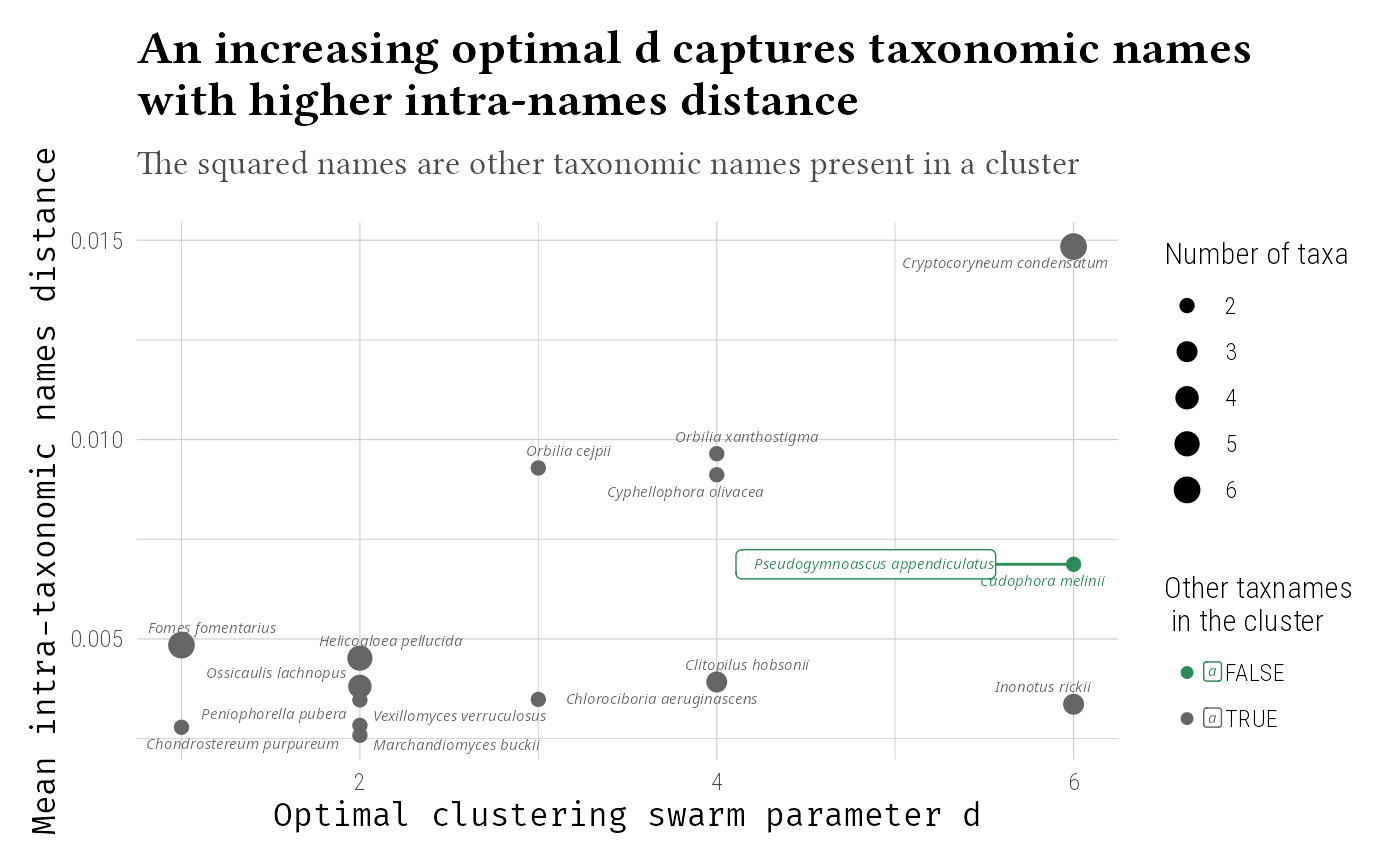
left_join(intra_taxn_dist, sbc_clusters$d_per_taxnames, by = "taxnames") |>
  mutate(is_na_optimal_d = is.na(optimal_d)) |>
  filter(!is.na(mean_dist)) |>
  ggplot(aes(x = mean_dist, y = is_na_optimal_d, color = optimal_d)) +
  geom_violin() +
  geom_jitter() +
  geom_vline(xintercept = 0.03, color = "red") +
  theme_idest()
Session information
#> R version 4.6.0 (2026-04-24)
#> Platform: x86_64-pc-linux-gnu
#> Running under: Pop!_OS 24.04 LTS
#>
#> Matrix products: default
#> BLAS:   /usr/lib/x86_64-linux-gnu/openblas-pthread/libblas.so.3
#> LAPACK: /usr/lib/x86_64-linux-gnu/openblas-pthread/libopenblasp-r0.3.26.so;  LAPACK version 3.12.0
#>
#> locale:
#>  [1] LC_CTYPE=en_US.UTF-8       LC_NUMERIC=C
#>  [3] LC_TIME=en_US.UTF-8        LC_COLLATE=en_US.UTF-8
#>  [5] LC_MONETARY=en_US.UTF-8    LC_MESSAGES=en_US.UTF-8
#>  [7] LC_PAPER=en_US.UTF-8       LC_NAME=C
#>  [9] LC_ADDRESS=C               LC_TELEPHONE=C
#> [11] LC_MEASUREMENT=en_US.UTF-8 LC_IDENTIFICATION=C
#>
#> time zone: Europe/Paris
#> tzcode source: system (glibc)
#>
#> attached base packages:
#> [1] stats     graphics  grDevices utils     datasets  methods   base
#>
#> other attached packages:
#> [1] taxinfo_0.1.2      MiscMetabar_0.16.8 dplyr_1.2.1        ggplot2_4.0.3
#> [5] phyloseq_1.56.0
#>
#> loaded via a namespace (and not attached):
#>  [1] ade4_1.7-24           tidyselect_1.2.1      farver_2.1.2
#>  [4] Biostrings_2.80.1     S7_0.2.2              bitops_1.0-9
#>  [7] divent_0.5-4          fastmap_1.2.0         RCurl_1.98-1.19
#> [10] digest_0.6.39         lifecycle_1.0.5       cluster_2.1.8.2
#> [13] survival_3.8-6        magrittr_2.0.5        compiler_4.6.0
#> [16] rlang_1.2.0           sass_0.4.10           tools_4.6.0
#> [19] igraph_2.3.2          yaml_2.3.12           data.table_1.18.4
#> [22] knitr_1.51            labeling_0.4.3        htmlwidgets_1.6.4
#> [25] plyr_1.8.9            RColorBrewer_1.1-3    withr_3.0.2
#> [28] purrr_1.2.2           BiocGenerics_0.58.1   desc_1.4.3
#> [31] grid_4.6.0            stats4_4.6.0          multtest_2.68.0
#> [34] biomformat_1.40.0     scales_1.4.0          iterators_1.0.14
#> [37] MASS_7.3-65           cli_3.6.6             rmarkdown_2.31
#> [40] vegan_2.7-5           crayon_1.5.3          ragg_1.5.2
#> [43] generics_0.1.4        otel_0.2.0            RcppParallel_5.1.11-2
#> [46] reshape2_1.4.5        pbapply_1.7-4         DBI_1.3.0
#> [49] ape_5.8-1             cachem_1.1.0          stringr_1.6.0
#> [52] splines_4.6.0         parallel_4.6.0        XVector_0.52.0
#> [55] vctrs_0.7.3           Matrix_1.7-5          jsonlite_2.0.0
#> [58] IRanges_2.46.0        S4Vectors_0.50.1      ggrepel_0.9.8
#> [61] systemfonts_1.3.2     foreach_1.5.2         rglobi_0.3.4
#> [64] jquerylib_0.1.4       tidyr_1.3.2           glue_1.8.1
#> [67] pkgdown_2.2.0         codetools_0.2-20      stringi_1.8.7
#> [70] gtable_0.3.6          tibble_3.3.1          pillar_1.11.1
#> [73] htmltools_0.5.9       Seqinfo_1.2.0         R6_2.6.1
#> [76] textshaping_1.0.5     Rdpack_2.6.6          evaluate_1.0.5
#> [79] lattice_0.22-9        Biobase_2.72.0        rbibutils_2.4.1
#> [82] DECIPHER_3.8.0        bslib_0.11.0          Rcpp_1.1.1-1.1
#> [85] nlme_3.1-169          permute_0.9-10        mgcv_1.9-4
#> [88] xfun_0.58             fs_2.1.0              pkgconfig_2.0.3