Alpha diversity analysis
Hill number
Numerous metrics of diversity exist. Hill numbers 1 is a kind of general framework for alpha diversity index.
Diversity profiles
profile_hill_pq() plots the Hill diversity profile
(diversity as a function of the order q) for each sample, or
for groups of samples merged via merge_sample_by.
data(data_fungi_mini)
dfm_rarefied <- rarefy_even_depth(data_fungi_mini, rngseed = 1, sample.size = 200)
p <- profile_hill_pq(dfm_rarefied)

p + no_legend()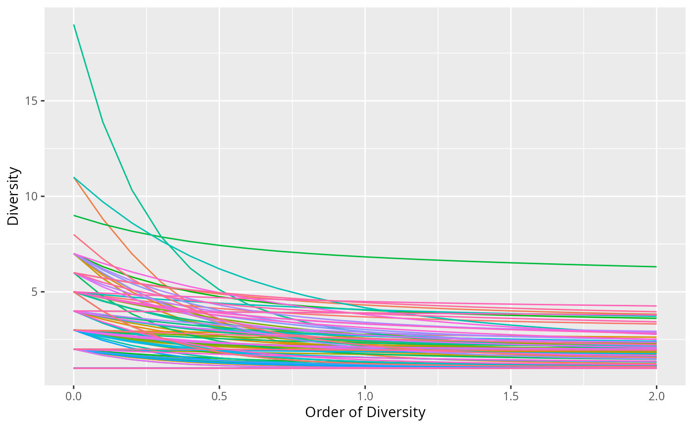
Hill diversity profiles per sample (data_fungi_mini)
profile_hill_pq(dfm_rarefied, merge_sample_by = "Height")
#> Warning in merge_samples2(physeq, merge_sample_by): `group` has missing values;
#> corresponding samples will be dropped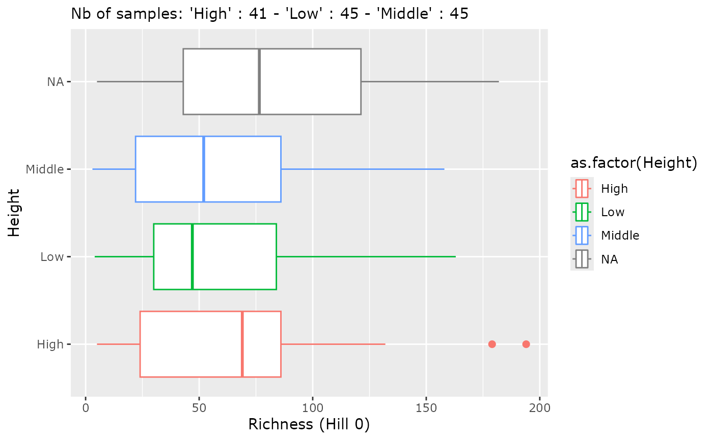
Hill diversity profiles merged by Height
Rarefaction curves
hill_acc_pq() plots Hill diversity accumulation
(rarefaction) curves — one per sample or per merged group — showing how
estimated diversity grows with sequencing depth.
hill_acc_pq(dfm_rarefied, q = 1, n_simulations = 5) + no_legend()
#> Warning: This manual palette can handle a maximum of 13 values. You have
#> supplied 89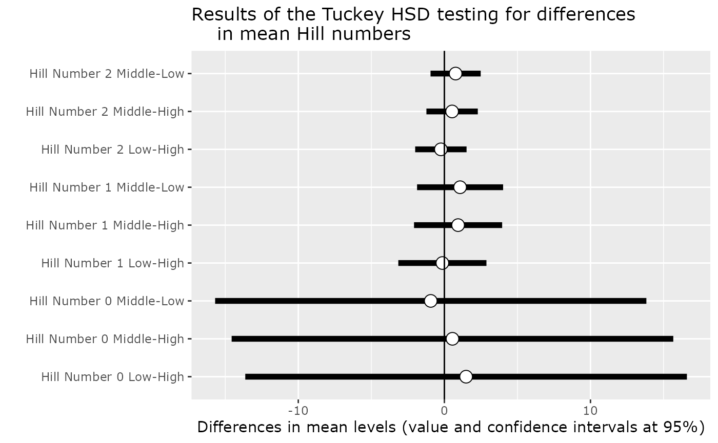
Rarefaction curves per sample (Hill order q = 1)
hill_acc_pq(dfm_rarefied, q = 0, merge_sample_by = "Height", n_simulations = 5)
#> Warning in merge_samples2(physeq, merge_sample_by): `group` has missing values;
#> corresponding samples will be dropped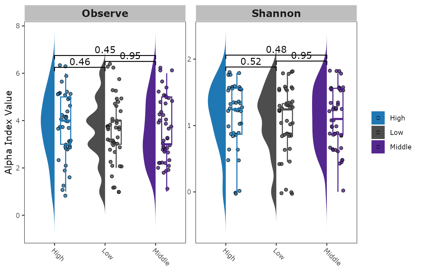
Rarefaction curves merged by Height (Hill order q = 0)
Test for difference in diversity (hill number)
One way to keep into account for difference in the number of sequences per samples is to use a Tukey test on a linear model with the square roots of the number of sequence as the first explanatory variable of the linear model 2.
p <- MiscMetabar::hill_pq(data_fungi, fact = "Height")
p$plot_Hill_0
Hill number 1
p$plot_tuckey
#> NULL
See also the tutorial of the microbiome package for an alternative using the non-parametric Kolmogorov-Smirnov test for two-group comparisons when there are no relevant covariates.
Alpha diversity using package MicrobiotaProcess
library("MicrobiotaProcess")
clean_pq(subset_samples_pq(data_fungi, !is.na(data_fungi@sam_data$Height))) %>%
  as.MPSE() %>%
  mp_cal_alpha() %>%
  mp_plot_alpha(.group = "Height")
#> Warning: `aes_string()` was deprecated in ggplot2 3.0.0.
#> ℹ Please use tidy evaluation idioms with `aes()`.
#> ℹ See also `vignette("ggplot2-in-packages")` for more information.
#> ℹ The deprecated feature was likely used in the MicrobiotaProcess package.
#>   Please report the issue at
#>   <https://github.com/YuLab-SMU/MicrobiotaProcess/issues>.
#> This warning is displayed once per session.
#> Call `lifecycle::last_lifecycle_warnings()` to see where this warning was
#> generated.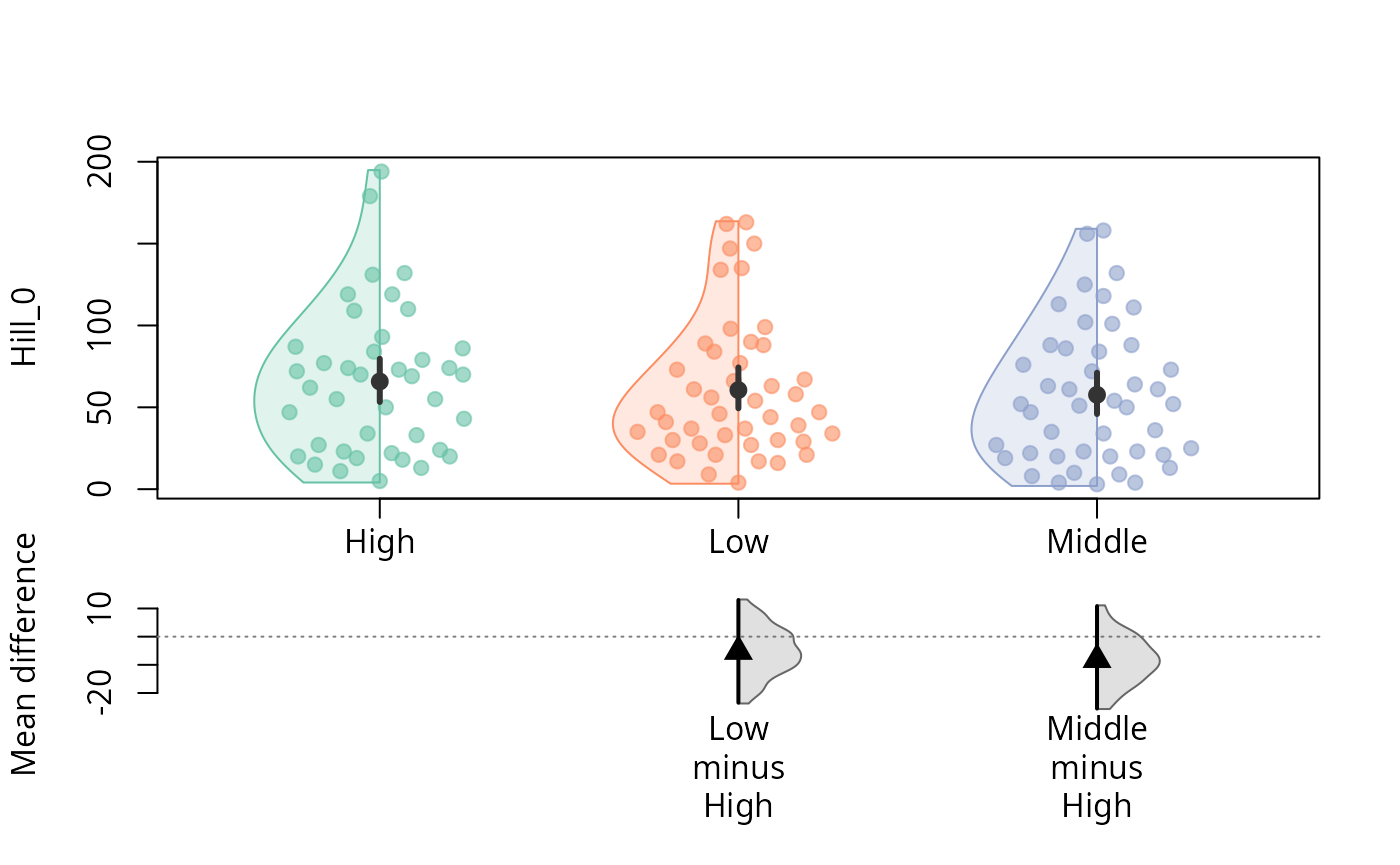
Estimation statistics framework
” Estimation statistics is a simple framework that avoids the pitfalls of significance testing. It uses familiar statistical concepts: means, mean differences, and error bars. More importantly, it focuses on the effect size of one’s experiment/intervention, as opposed to a false dichotomy engendered by P values. ” Citation from dabest documentation website.
Durga package
library("Durga")
psm <- psmelt_samples_pq(data_fungi)

durga_res <- DurgaDiff(Hill_0 ~ Time == 0, psm)
DurgaPlot(durga_res)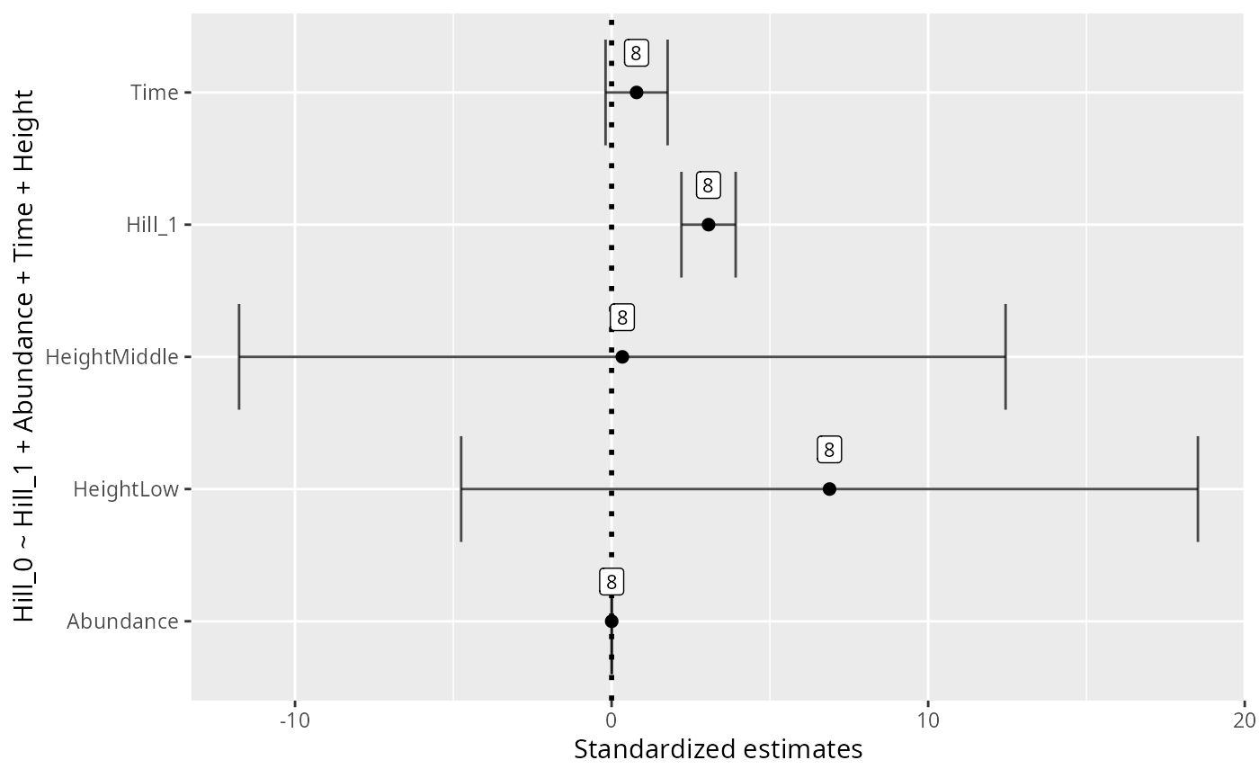
durga_pq <- function(physeq, formula, plot = FALSE) {
  verify_pq(physeq)
  psm <- psmelt_samples_pq(physeq)
  res_durga <- DurgaDiff(formula, psm)
  if (plot) {
    p <- DurgaPlot(res_durga)
    invisible(p)
  } else {
    return(res_durga)
  }
}

durga_pq(data_fungi, Hill_0 ~ Height, plot = TRUE)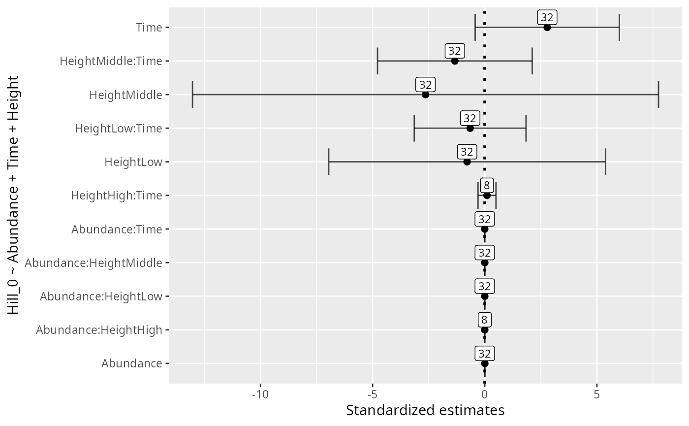
durga_pq(data_fungi, Hill_0 ~ Time + Height, plot = TRUE)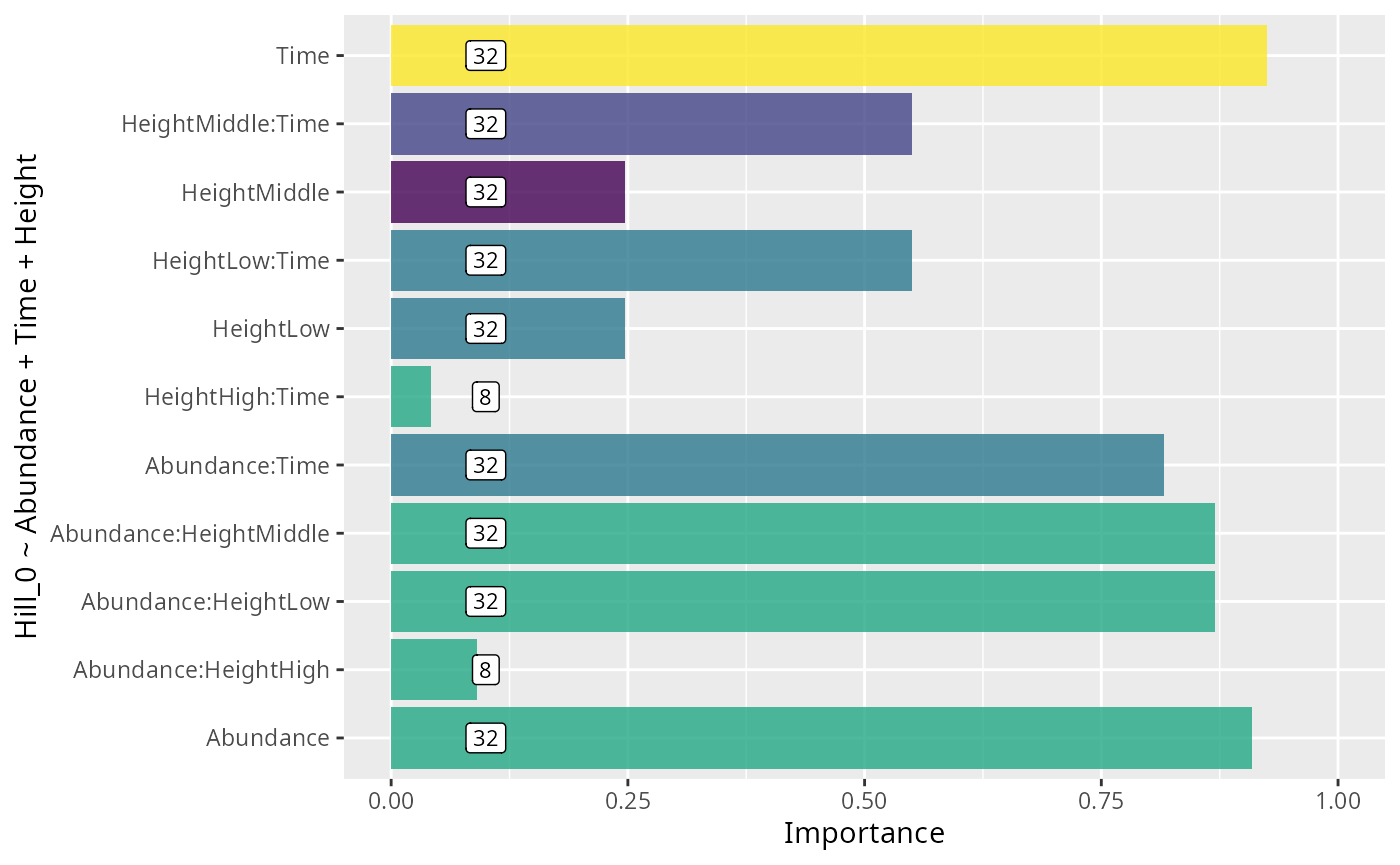
durga_pq(data_fungi, Hill_0 ~ Time == 0, plot = TRUE)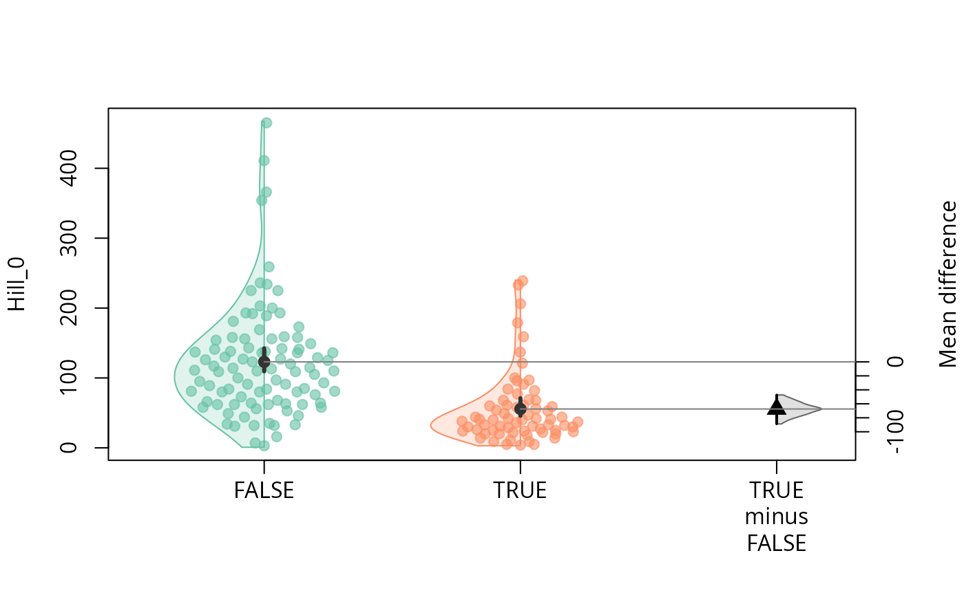
durga_pq(data_fungi, Hill_1 ~ Time == 0, plot = TRUE)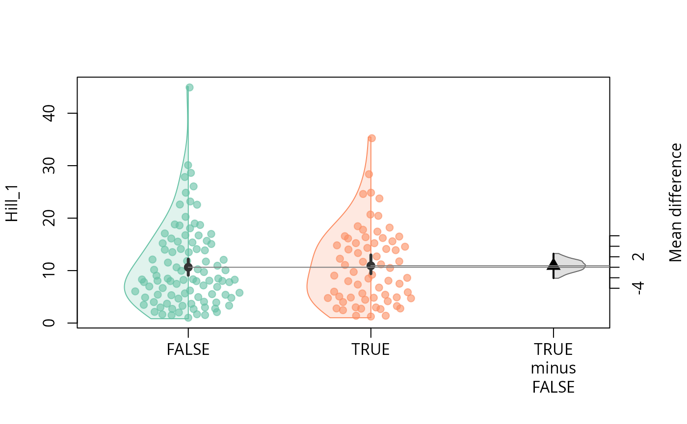
durga_pq(data_fungi, Hill_2 ~ Time == 0, plot = TRUE)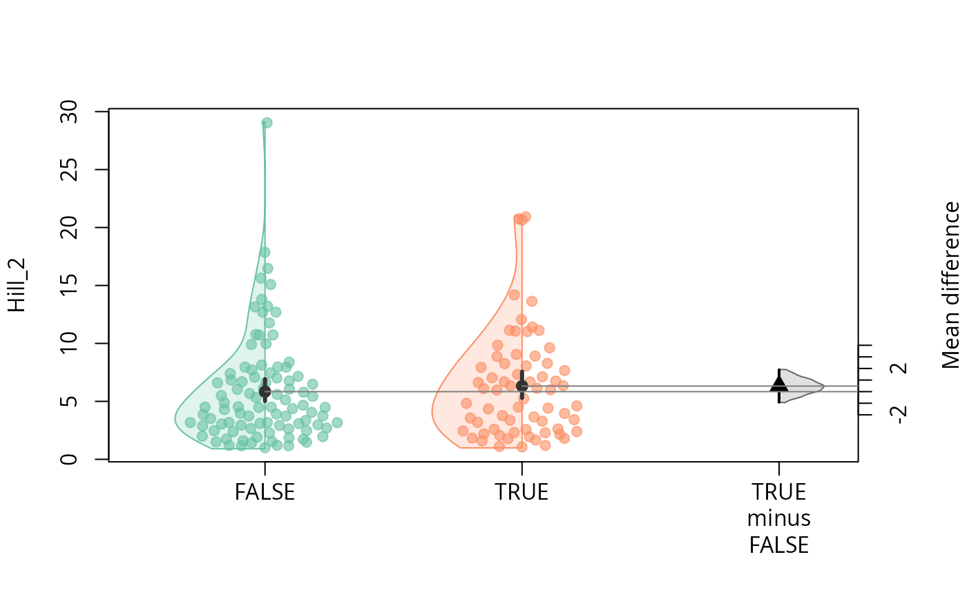
dabest R package
library("dabestr")
psm <- psmelt_samples_pq(data_fungi)

load(
  data = psm,
  x = Height,
  y = Hill_2,
  idx = list(c("Low", "Middle", "High"))
) %>%
  mean_diff() |>
  dabest_plot(swarm_label = "Hill_2")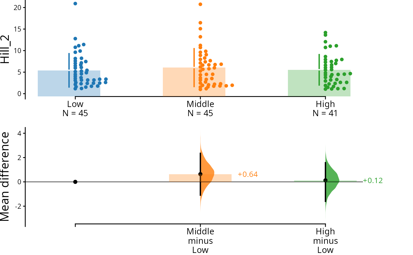
psm |>
  mutate(Time_is_0 = Time == 0) |>
  load(
    x = Time_is_0,
    y = Hill_0,
    idx = list(c("TRUE", "FALSE"))
  ) %>%
  mean_diff() |>
  dabest_plot(swarm_label = "Hill_0")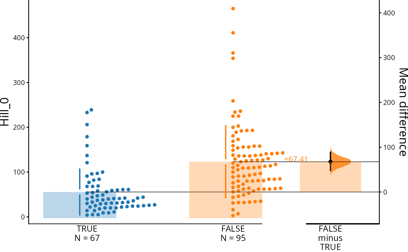
Effect of samples variables on alpha diversity using automated model selection and multimodel inference with (G)LMs
From the help of glmulti package :
glmulti finds what are the n best models (the confidence set of models) among all possible models (the candidate set, as specified by the user). Models are fitted with the specified fitting function (default is glm) and are ranked with the specified Information Criterion (default is aicc). The best models are found either through exhaustive screening of the candidates, or using a genetic algorithm, which allows very large candidate sets to be addressed. The output can be used for model selection, variable selection, and multimodel inference.
library("glmulti")
formula <- "Hill_0 ~ Hill_1 + Abundance + Time + Height"
res_glmulti <-
  glmutli_pq(data_fungi_mini, formula = formula, level = 1)
#> Initialization...
#> TASK: Exhaustive screening of candidate set.
#> Fitting...
#> Completed.
res_glmulti
#>                  estimates unconditional_interval nb_model importance
#> Abundance     0.0002425004           4.049862e-09        8  0.9976746
#> Hill_1        1.4818202876           1.144356e-01        8  0.9996675
#> Time          0.0202445718           3.271583e-03        8  1.0000000
#> HeightLow    -0.0685647506           6.111797e-01        8  1.0000000
#> HeightMiddle  0.1905543547           6.885434e-01        8  1.0000000
#>                     alpha     variable
#> Abundance    0.0001269354    Abundance
#> Hill_1       0.6748363040       Hill_1
#> Time         0.1141042429         Time
#> HeightLow    1.5596025795    HeightLow
#> HeightMiddle 1.6553735697 HeightMiddle

ggplot(data = res_glmulti, aes(x = estimates, y = variable)) +
  geom_point(
    size = 2,
    alpha = 1,
    show.legend = FALSE
  ) +
  geom_vline(
    xintercept = 0,
    linetype = "dotted",
    linewidth = 1
  ) +
  geom_errorbar(
    aes(xmin = estimates - alpha, xmax = estimates + alpha),
    width = 0.8,
    position = position_dodge(width = 0.8),
    alpha = 0.7,
    show.legend = FALSE
  ) +
  geom_label(aes(label = nb_model), nudge_y = 0.3, size = 3) +
  xlab("Standardized estimates") +
  ylab(formula)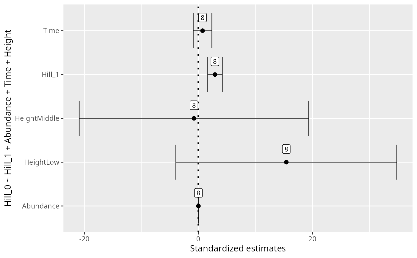
ggplot(data = res_glmulti, aes(
  x = importance,
  y = as.factor(variable),
  fill = estimates
)) +
  geom_bar(
    stat = "identity",
    show.legend = FALSE,
    alpha = 0.8
  ) +
  xlim(c(0, 1)) +
  geom_label(aes(label = nb_model, x = 0.1),
    size = 3,
    fill = "white"
  ) +
  scale_fill_viridis_b() +
  xlab("Importance") +
  ylab(formula)
#> Warning: Removed 2 rows containing missing values or values outside the scale range
#> (`geom_bar()`).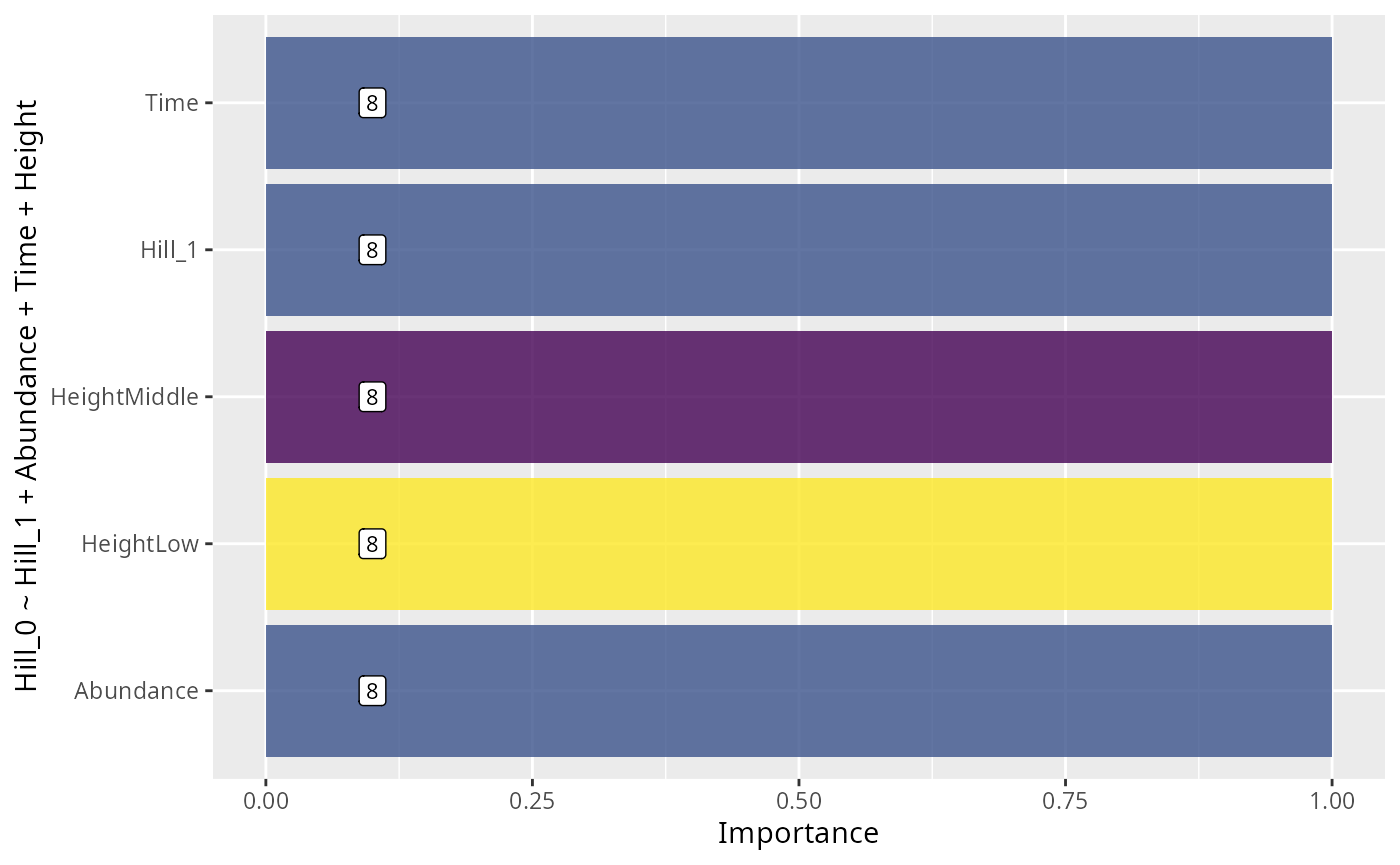
formula <- "Hill_0 ~ Abundance + Time + Height"
res_glmulti_interaction <-
  glmutli_pq(data_fungi_mini, formula = formula, level = 2)
#> Initialization...
#> TASK: Exhaustive screening of candidate set.
#> Fitting...
#>
#> After 50 models:
#> Best model: Hill_0~1+Abundance+Time+Time:Abundance+Height:Abundance
#> Crit= 380.266307886255
#> Mean crit= 439.149731147241
#> Completed.
res_glmulti_interaction
#>                            estimates unconditional_interval nb_model
#> HeightHigh:Time         1.021021e-03           4.896053e-06        8
#> Abundance:HeightHigh    1.444574e-06           1.376218e-11        8
#> HeightLow              -2.818502e-01           2.975283e-01       32
#> HeightMiddle           -2.284000e-01           2.804621e-01       32
#> HeightLow:Time         -4.802362e-02           7.037018e-03       32
#> HeightMiddle:Time      -5.451488e-02           8.777216e-03       32
#> Abundance:HeightLow     9.952410e-05           2.196739e-08       32
#> Abundance:HeightMiddle  1.942462e-04           3.617651e-08       32
#> Time                    1.927954e-01           1.152254e-02       32
#> Abundance               4.367041e-04           3.508660e-08       32
#> Abundance:Time         -3.131657e-05           1.596068e-10       32
#>                         importance        alpha               variable
#> HeightHigh:Time        0.006596239 4.348738e-03        HeightHigh:Time
#> Abundance:HeightHigh   0.014891518 7.317402e-06   Abundance:HeightHigh
#> HeightLow              0.293275977 1.076681e+00              HeightLow
#> HeightMiddle           0.293275977 1.046605e+00           HeightMiddle
#> HeightLow:Time         0.409654935 1.655170e-01         HeightLow:Time
#> HeightMiddle:Time      0.409654935 1.848108e-01      HeightMiddle:Time
#> Abundance:HeightLow    0.671985280 2.935384e-04    Abundance:HeightLow
#> Abundance:HeightMiddle 0.671985280 3.755994e-04 Abundance:HeightMiddle
#> Time                   0.900282159 2.125915e-01                   Time
#> Abundance              0.933935731 3.708996e-04              Abundance
#> Abundance:Time         0.967098115 2.508155e-05         Abundance:Time

ggplot(data = res_glmulti_interaction, aes(x = estimates, y = variable)) +
  geom_point(
    size = 2,
    alpha = 1,
    show.legend = FALSE
  ) +
  geom_vline(
    xintercept = 0,
    linetype = "dotted",
    linewidth = 1
  ) +
  geom_errorbar(
    aes(xmin = estimates - alpha, xmax = estimates + alpha),
    width = 0.8,
    position = position_dodge(width = 0.8),
    alpha = 0.7,
    show.legend = FALSE
  ) +
  geom_label(aes(label = nb_model), nudge_y = 0.3, size = 3) +
  xlab("Standardized estimates") +
  ylab(formula)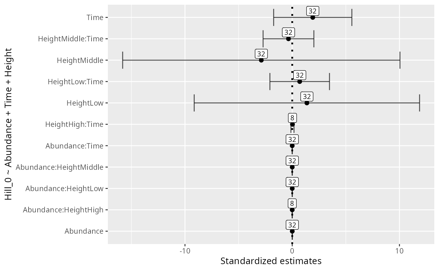
ggplot(data = res_glmulti_interaction, aes(
  x = importance,
  y = as.factor(variable),
  fill = estimates
)) +
  geom_bar(
    stat = "identity",
    show.legend = FALSE,
    alpha = 0.8
  ) +
  xlim(c(0, 1)) +
  geom_label(aes(label = nb_model, x = 0.1),
    size = 3,
    fill = "white"
  ) +
  scale_fill_viridis_b() +
  xlab("Importance") +
  ylab(formula)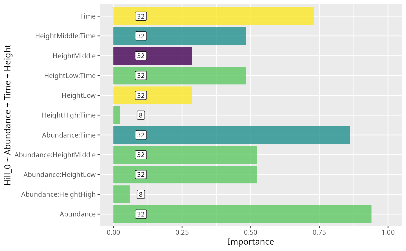
Session information
sessionInfo()
#> R version 4.6.0 (2026-04-24)
#> Platform: x86_64-pc-linux-gnu
#> Running under: Pop!_OS 24.04 LTS
#>
#> Matrix products: default
#> BLAS:   /usr/lib/x86_64-linux-gnu/openblas-pthread/libblas.so.3
#> LAPACK: /usr/lib/x86_64-linux-gnu/openblas-pthread/libopenblasp-r0.3.26.so;  LAPACK version 3.12.0
#>
#> locale:
#>  [1] LC_CTYPE=en_US.UTF-8          LC_NUMERIC=C
#>  [3] LC_TIME=en_US.UTF-8           LC_COLLATE=en_US.UTF-8
#>  [5] LC_MONETARY=en_US.UTF-8       LC_MESSAGES=en_US.UTF-8
#>  [7] LC_PAPER=en_US.UTF-8          LC_NAME=en_US.UTF-8
#>  [9] LC_ADDRESS=en_US.UTF-8        LC_TELEPHONE=en_US.UTF-8
#> [11] LC_MEASUREMENT=en_US.UTF-8    LC_IDENTIFICATION=en_US.UTF-8
#>
#> time zone: Europe/Paris
#> tzcode source: system (glibc)
#>
#> attached base packages:
#> [1] stats     graphics  grDevices utils     datasets  methods   base
#>
#> other attached packages:
#>  [1] glmulti_1.0.8            leaps_3.2                rJava_1.0-18
#>  [4] dabestr_2025.3.15        Durga_2.1.0              MicrobiotaProcess_1.24.0
#>  [7] divent_0.5-4             Rcpp_1.1.1-1.1           MiscMetabar_0.16.8
#> [10] dplyr_1.2.1              ggplot2_4.0.3            phyloseq_1.56.0
#>
#> loaded via a namespace (and not attached):
#>   [1] libcoin_1.0-12              RColorBrewer_1.1-3
#>   [3] jsonlite_2.0.0              magrittr_2.0.5
#>   [5] TH.data_1.1-5               modeltools_0.2-24
#>   [7] ggbeeswarm_0.7.3            farver_2.1.2
#>   [9] rmarkdown_2.31              fs_2.1.0
#>  [11] ragg_1.5.2                  vctrs_0.7.3
#>  [13] multtest_2.68.0             ggtree_4.2.0
#>  [15] htmltools_0.5.9             S4Arrays_1.12.0
#>  [17] SparseArray_1.12.2          gridGraphics_0.5-1
#>  [19] sass_0.4.10                 bslib_0.11.0
#>  [21] htmlwidgets_1.6.4           desc_1.4.3
#>  [23] plyr_1.8.9                  sandwich_3.1-1
#>  [25] zoo_1.8-15                  cachem_1.1.0
#>  [27] igraph_2.3.2                lifecycle_1.0.5
#>  [29] iterators_1.0.14            pkgconfig_2.0.3
#>  [31] Matrix_1.7-5                R6_2.6.1
#>  [33] fastmap_1.2.0               rbibutils_2.4.1
#>  [35] MatrixGenerics_1.24.0       digest_0.6.39
#>  [37] aplot_0.2.9                 ggnewscale_0.5.2
#>  [39] patchwork_1.3.2             S4Vectors_0.50.1
#>  [41] textshaping_1.0.5           GenomicRanges_1.64.0
#>  [43] vegan_2.7-5                 labeling_0.4.3
#>  [45] abind_1.4-8                 mgcv_1.9-4
#>  [47] compiler_4.6.0              fontquiver_0.2.1
#>  [49] withr_3.0.2                 S7_0.2.2
#>  [51] ggsignif_0.6.4              MASS_7.3-65
#>  [53] rappdirs_0.3.4              DelayedArray_0.38.2
#>  [55] biomformat_1.40.0           ggsci_5.0.0
#>  [57] permute_0.9-10              tools_4.6.0
#>  [59] vipor_0.4.7                 otel_0.2.0
#>  [61] beeswarm_0.4.0              ape_5.8-1
#>  [63] glue_1.8.1                  nlme_3.1-169
#>  [65] grid_4.6.0                  cluster_2.1.8.2
#>  [67] reshape2_1.4.5              ade4_1.7-24
#>  [69] generics_0.1.4              gtable_0.3.6
#>  [71] tidyr_1.3.2                 data.table_1.18.4
#>  [73] coin_1.4-3                  XVector_0.52.0
#>  [75] BiocGenerics_0.58.1         ggrepel_0.9.8
#>  [77] foreach_1.5.2               pillar_1.11.1
#>  [79] stringr_1.6.0               yulab.utils_0.2.4
#>  [81] splines_4.6.0               treeio_1.36.1
#>  [83] lattice_0.22-9              survival_3.8-6
#>  [85] tidyselect_1.2.1            fontLiberation_0.1.0
#>  [87] Biostrings_2.80.1           knitr_1.51
#>  [89] fontBitstreamVera_0.1.1     gridExtra_2.3
#>  [91] IRanges_2.46.0              Seqinfo_1.2.0
#>  [93] SummarizedExperiment_1.42.0 ggtreeExtra_1.22.0
#>  [95] stats4_4.6.0                xfun_0.58
#>  [97] Biobase_2.72.0              matrixStats_1.5.0
#>  [99] stringi_1.8.7               lazyeval_0.2.3
#> [101] ggfun_0.2.0                 yaml_2.3.12
#> [103] boot_1.3-32                 evaluate_1.0.5
#> [105] codetools_0.2-20            effsize_0.8.1
#> [107] gdtools_0.5.1               tibble_3.3.1
#> [109] ggplotify_0.1.3             cli_3.6.6
#> [111] RcppParallel_5.1.11-2       systemfonts_1.3.2
#> [113] Rdpack_2.6.6                jquerylib_0.1.4
#> [115] parallel_4.6.0              pkgdown_2.2.0
#> [117] ggh4x_0.3.1                 ggstar_1.0.6
#> [119] viridisLite_0.4.3           mvtnorm_1.4-0
#> [121] tidytree_0.4.7              ggiraph_0.9.6
#> [123] scales_1.4.0                purrr_1.2.2
#> [125] crayon_1.5.3                rlang_1.2.0
#> [127] cowplot_1.2.0               multcomp_1.4-30