Re-clustering ASVs
ASV (stands for Amplicon Sequence Variant; also called ESV for Exact Amplicon Variant) is a DNA sequence obtained from high-throughput analysis of marker genes. OTU (stands for Operational Taxonomic Unit) is a group of closely related individuals created by clustering sequences based on a threshold of similarity. An ASV is a special case of an OTU with a similarity threshold of 100%. A third concept is the zero-radius OTU zOTU (Edgar 2016) which is the same concept than ASV but compute with other softwares than dada (e.g. vsearch).
The choice between ASV and OTU is important because they lead to different results (Joos et al. (2020), Box 2 in Tedersoo et al. (2022), Chiarello et al. (2022)). Most articles recommend making a choice depending on the question (mclaren2018?), For example, ASV may be better than OTU for describing a group of very closely related species. In addition, ASV are comparable across different datasets (obtained using identical marker genes). (fasolo2024?) showed that that the OTUs clustering of 16S rDNA proportionally led to a marked underestimation of the ecological indicators values for species diversity and to a distorted behaviour of the dominance and evenness indexes with respect to the direct use of the ASV data. On the other hand, Tedersoo et al. (2022) report that ASV approaches overestimate the richness of common fungal species (due to haplotype variation), but underestimate the richness of rare species. They recommend the OTUs approach in metabarcoding analyses of fungal communities. Finally, Kauserud (2023) argues that the ASV term falls within the original OTU term and recommends adopting only the OTU terms, but with a concise and clear report on how the OTUs were generated.
Recent articles (Forster et al. 2019; Antich et al. 2021; Brandt et al. 2021) propose to use both approaches together. They recommend (i) using ASV to denoise the dataset and (ii) for some questions, clustering the ASV sequences into OTUs. (García-García et al. 2019) used both concept to demonstrate that ecotypes (ASV within OTUs) are adapted to different values of environmental factors favoring the persistence of OTU across changing environmental conditions.
The goal of the function asv2otu() is to facilitate the
reclustering of ASV into OTU, using either the
DECIPHER::Clusterize function from R or the vsearch software.
As part of the Metabarcoding Data Toolkit (MDT), the Global Biodiversity Information Facility (GBIF) recommend “sharing unclustered (but denoised) amplicon sequence variants (ASVs) from e.g. the dada2 pipeline” for Illumina MiSeq plateform. They args that this approach keeps data maximally interoperable with data from other studies, compared to clustering into broader (e.g. 97% similarity) OTUs where the representative sequence of the same OTU may be picked differently between datasets and algorithms.
Using decipher or Vsearch algorithm
data(data_fungi_sp_known)
otu <- asv2otu(data_fungi_sp_known, method = "clusterize")
#> Partitioning sequences by 5-mer similarity:
#> ================================================================================
#>
#> Time difference of 0.2 secs
#>
#> Sorting by relatedness within 651 groups:
#> Clustering sequences by 9-mer similarity:
#> ================================================================================
#>
#> Time difference of 1.74 secs
#>
#> Clusters via relatedness sorting: 100% (0% exclusively)
#> Clusters via rare 5-mers: 100% (0% exclusively)
#> Estimated clustering effectiveness: 100%
otu_vs <- asv2otu(data_fungi_sp_known, method = "vsearch")The vsearch method requires the installation of Vsearch.
summary_plot_pq(data_fungi_sp_known)
summary_plot_pq(otu)
Using lulu algorithm (link to LULU article)
Another post-clustering transformation method is implemented in
lulu_pq(), which uses Frøslev et al.
(2017)’s method for curation of DNA amplicon data. The aim is
more to clean non-biological information than to make explicitly less
clusters. For examples, Brandt et al.
(2021) clustered amplicon sequence variants (ASVs) into
operational taxonomic units (OTUs) with swarm and choose to curate
ASVs/OTUs using LULU. We recommend to use mumu a C++
re-implementation of LULU by Frédéric Mahé.
summary_plot_pq(data_fungi_sp_known)
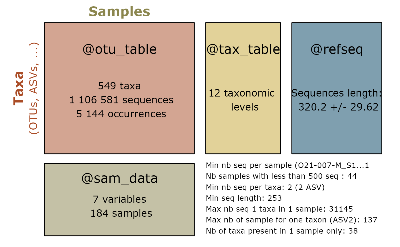
summary_plot_pq(lulu_res$new_physeq)
Tracking number of samples, sequences and clusters
track_wkflow(list(
  "Raw data" = data_fungi_sp_known,
  "OTU" = otu,
  "OTU_vsearch" = otu_vs,
  "LULU" = lulu_res[[1]]
))
#>             nb_sequences nb_clusters nb_samples
#> Raw data         1106581         651        185
#> OTU              1106581         363        185
#> OTU_vsearch      1106581         362        185
#> LULU             1106581         549        185
Session information
sessionInfo()
#> R version 4.5.2 (2025-10-31)
#> Platform: x86_64-pc-linux-gnu
#> Running under: Pop!_OS 24.04 LTS
#>
#> Matrix products: default
#> BLAS:   /usr/lib/x86_64-linux-gnu/blas/libblas.so.3.12.0
#> LAPACK: /usr/lib/x86_64-linux-gnu/lapack/liblapack.so.3.12.0  LAPACK version 3.12.0
#>
#> locale:
#>  [1] LC_CTYPE=fr_FR.UTF-8       LC_NUMERIC=C
#>  [3] LC_TIME=fr_FR.UTF-8        LC_COLLATE=fr_FR.UTF-8
#>  [5] LC_MONETARY=fr_FR.UTF-8    LC_MESSAGES=fr_FR.UTF-8
#>  [7] LC_PAPER=fr_FR.UTF-8       LC_NAME=C
#>  [9] LC_ADDRESS=C               LC_TELEPHONE=C
#> [11] LC_MEASUREMENT=fr_FR.UTF-8 LC_IDENTIFICATION=C
#>
#> time zone: Europe/Paris
#> tzcode source: system (glibc)
#>
#> attached base packages:
#> [1] stats     graphics  grDevices utils     datasets  methods   base
#>
#> other attached packages:
#> [1] MiscMetabar_0.14.6 purrr_1.2.1        dplyr_1.2.0        dada2_1.38.0
#> [5] Rcpp_1.1.1         ggplot2_4.0.2      phyloseq_1.54.0
#>
#> loaded via a namespace (and not attached):
#>   [1] DBI_1.2.3                   bitops_1.0-9
#>   [3] pbapply_1.7-4               deldir_2.0-4
#>   [5] permute_0.9-10              rlang_1.1.7
#>   [7] magrittr_2.0.4              ade4_1.7-23
#>   [9] otel_0.2.0                  matrixStats_1.5.0
#>  [11] compiler_4.5.2              mgcv_1.9-4
#>  [13] png_0.1-8                   systemfonts_1.3.1
#>  [15] vctrs_0.7.1                 reshape2_1.4.5
#>  [17] stringr_1.6.0               pwalign_1.6.0
#>  [19] pkgconfig_2.0.3             crayon_1.5.3
#>  [21] fastmap_1.2.0               XVector_0.50.0
#>  [23] labeling_0.4.3              Rsamtools_2.26.0
#>  [25] rmarkdown_2.30              ragg_1.5.0
#>  [27] xfun_0.56                   cachem_1.1.0
#>  [29] cigarillo_1.0.0             jsonlite_2.0.0
#>  [31] biomformat_1.38.0           rhdf5filters_1.22.0
#>  [33] DelayedArray_0.36.0         Rhdf5lib_1.32.0
#>  [35] BiocParallel_1.44.0         jpeg_0.1-11
#>  [37] parallel_4.5.2              cluster_2.1.8.2
#>  [39] R6_2.6.1                    bslib_0.10.0
#>  [41] stringi_1.8.7               RColorBrewer_1.1-3
#>  [43] GenomicRanges_1.62.1        jquerylib_0.1.4
#>  [45] Seqinfo_1.0.0               SummarizedExperiment_1.40.0
#>  [47] iterators_1.0.14            knitr_1.51
#>  [49] DECIPHER_3.6.0              IRanges_2.44.0
#>  [51] Matrix_1.7-4                splines_4.5.2
#>  [53] igraph_2.2.1                tidyselect_1.2.1
#>  [55] abind_1.4-8                 yaml_2.3.12
#>  [57] vegan_2.7-2                 codetools_0.2-20
#>  [59] hwriter_1.3.2.1             lattice_0.22-9
#>  [61] tibble_3.3.1                plyr_1.8.9
#>  [63] Biobase_2.70.0              withr_3.0.2
#>  [65] ShortRead_1.68.0            S7_0.2.1
#>  [67] evaluate_1.0.5              desc_1.4.3
#>  [69] survival_3.8-6              RcppParallel_5.1.11-1
#>  [71] Biostrings_2.78.0           pillar_1.11.1
#>  [73] MatrixGenerics_1.22.0       foreach_1.5.2
#>  [75] stats4_4.5.2                generics_0.1.4
#>  [77] S4Vectors_0.48.0            scales_1.4.0
#>  [79] glue_1.8.0                  tools_4.5.2
#>  [81] interp_1.1-6                data.table_1.18.2.1
#>  [83] GenomicAlignments_1.46.0    fs_1.6.6
#>  [85] rhdf5_2.54.1                grid_4.5.2
#>  [87] ape_5.8-1                   latticeExtra_0.6-31
#>  [89] nlme_3.1-168                cli_3.6.5
#>  [91] textshaping_1.0.4           S4Arrays_1.10.1
#>  [93] gtable_0.3.6                sass_0.4.10
#>  [95] digest_0.6.39               BiocGenerics_0.56.0
#>  [97] SparseArray_1.10.8          htmlwidgets_1.6.4
#>  [99] farver_2.1.2                htmltools_0.5.9
#> [101] pkgdown_2.2.0               multtest_2.66.0
#> [103] lifecycle_1.0.5             MASS_7.3-65