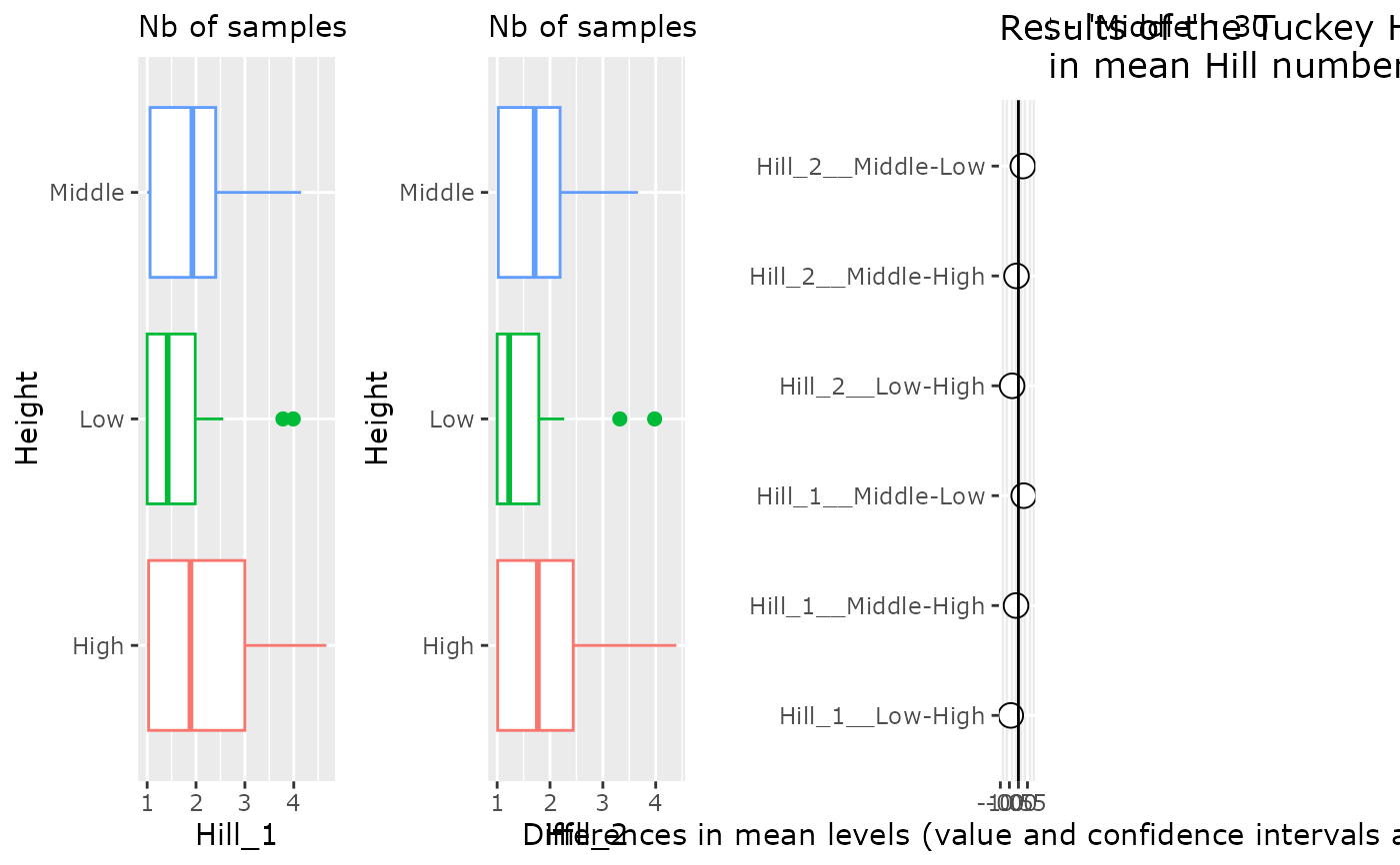
Graphical representation of hill number 0, 1 and 2 across a factor

Hill numbers are the number of equiprobable species giving the same diversity value as the observed distribution. The Hill number 0 correspond to Species richness), the Hill number 1 to the exponential of Shannon Index and the Hill number 2 to the inverse of Simpson Index)

Note that (if correction_for_sample_size is TRUE, default behavior) this function use a sqrt of the read numbers in the linear model in order to correct for uneven sampling depth. This correction is only done before tuckey HSD plot and do not change the hill number computed.

Usage

hill_pq(
  physeq,
  fact = NULL,
  variable = NULL,
  hill_scales = c(0, 1, 2),
  color_fac = NA,
  letters = FALSE,
  add_points = FALSE,
  add_info = TRUE,
  one_plot = FALSE,
  plot_with_tuckey = TRUE,
  correction_for_sample_size = TRUE,
  na_remove = TRUE
)

Arguments

physeq: (required): a phyloseq-class object obtained using the phyloseq package.
fact: (required): The variable to test. Must be present in the sam_data slot of the physeq object.
variable: : Alias for factor. Kept only for backward compatibility.
hill_scales: (a vector of integer) The list of q values to compute the hill number H^q. If Null, no hill number are computed. Default value compute the Hill number 0 (Species richness), the Hill number 1 (exponential of Shannon Index) and the Hill number 2 (inverse of Simpson Index).
color_fac: (optional): The variable to color the barplot. For ex. same as fact. Not very useful because ggplot2 plot colors can be change using scale_color_XXX() function.
letters: (optional, default=FALSE): If set to TRUE, the plot show letters based on p-values for comparison. Use the multcompLetters function from the package multcompLetters. BROKEN for the moment. Note that na values in The variable param need to be removed (see examples) to use letters.
add_points: (logical): add jitter point on boxplot
add_info: (logical, default TRUE) Do we add a subtitle with information about the number of samples per modality ?
one_plot: (logical, default FALSE) If TRUE, return a unique plot with the four plot inside using the patchwork package. Note that if letters and one_plot are both TRUE, tuckey HSD results are discarded from the unique plot. In that case, use one_plot = FALSE to see the tuckey HSD results in the fourth plot of the resulting list.
plot_with_tuckey: (logical, default TRUE). If one_plot is set to TRUE and letters to FALSE, allow to discard the tuckey plot part with plot_with_tuckey = FALSE
correction_for_sample_size: (logical, default TRUE) This function use a sqrt of the read numbers in the linear model in order to correct for uneven sampling depth in the Tuckey TEST. This params do not change value of Hill number but only the test associated values (including the pvalues). To rarefy samples, you may use the function phyloseq::rarefy_even_depth().
na_remove: (logical, default TRUE) Do we remove samples with NA in the factor fact ? Note that na_remove is always TRUE when using letters = TRUE

Value

Either an unique ggplot2 object (if one_plot is TRUE) or a list of 4 ggplot2 plot:

plot_Hill_0 : the boxplot of Hill number 0 (= species richness) against the variable
plot_Hill_1 : the boxplot of Hill number 1 (= Shannon index) against the variable
plot_Hill_2 : the boxplot of Hill number 2 (= Simpson index) against the variable
plot_tuckey : plot the result of the Tuckey HSD test

Author

Adrien Taudière

Examples


p <- hill_pq(data_fungi_mini, "Height", hill_scales = 1:2)
p_h1 <- p[[1]] + theme(legend.position = "none")
p_h2 <- p[[2]] + theme(legend.position = "none")
multiplot(plotlist = list(p_h1, p_h2, p[[3]]), cols = 4)

# \donttest{
if (requireNamespace("multcompView")) {
  p2 <- hill_pq(data_fungi, "Time",
    correction_for_sample_size = FALSE,
    letters = TRUE, add_points = TRUE, plot_with_tuckey = FALSE
  )
  if (requireNamespace("patchwork")) {
    patchwork::wrap_plots(p2, guides = "collect")
  }
  # Artificially modify data_fungi to force alpha-diversity effect
  data_fungi_modif <- clean_pq(subset_samples_pq(data_fungi, !is.na(data_fungi@sam_data$Height)))
  data_fungi_modif@otu_table[data_fungi_modif@sam_data$Height == "High", ] <-
    data_fungi_modif@otu_table[data_fungi_modif@sam_data$Height == "High", ] +
    sample(c(rep(0, ntaxa(data_fungi_modif) / 2), rep(100, ntaxa(data_fungi_modif) / 2)))
  p3 <- hill_pq(data_fungi_modif, "Height", letters = TRUE)
  p3[[1]]
}
#> Taxa are now in rows.
#> Joining with `by = join_by(Time)`
#> Joining with `by = join_by(Time)`
#> Joining with `by = join_by(Time)`
#> Cleaning suppress 144 taxa and 0 samples.
#> Taxa are now in rows.
#> Joining with `by = join_by(Height)`
#> Joining with `by = join_by(Height)`
#> Joining with `by = join_by(Height)`

# }

References

Alberdi, A., & Gilbert, M. T. P. (2019). A guide to the application of Hill numbers to DNA-based diversity analyses. Molecular Ecology Resources. doi:10.1111/1755-0998.13014
Calderón-Sanou, I., Münkemüller, T., Boyer, F., Zinger, L., & Thuiller, W. (2019). From environmental DNA sequences to ecological conclusions: How strong is the influence of methodological choices? Journal of Biogeography, 47. doi:10.1111/jbi.13681
Examples
data_f <- prune_samples(
sample_names(data_fungi_mini)[1:20],
data_fungi_mini
)
p <- hill_pq(data_f, "Height", q = c(0, 1))
#> 2 out of 2 Hill scales do not show any global trends with you factor Height. Tuckey HSD plot is not informative for those Hill scales. Letters are not printed for those Hill scales
p[[1]] + theme(legend.position = "none")
if (FALSE) { # \dontrun{